A Brief Introduction to q and KDB-X
Welcome! This page introduces the basics of q and KDB‑X. Through practical examples, you'll learn how to create data, run queries, and understand the core principles of q's concise syntax and high‑performance design. No prior knowledge is required. You'll pick up the essentials as you work through the exercises.
KDB-X is a powerful ecosystem built on top of q. The q language is a concise, expressive, dynamically typed, interpreted programming language with a built-in database engine optimized for streaming, real-time, and historical data. By bringing the application logic and data together, KDB-X eliminates the overhead associated with complex multi-layer architectures.
If you don't have KDB-X installed yet, follow this quick install KDB-X guide.
Launch q
In your terminal, type q to start an interactive session. When the q) prompt appears, the interpreter is ready.
q
KDB-X 5.0.20251113 2025.11.13 Copyright (C) 1993-2025 Kx Systems
...

q)
Note
The code examples below are cumulative. Each section assumes the variables and state defined in all preceding sections are still in your active q session.
Standard constructs
Like most languages, q allows you to create scalars, lists, and dictionaries, and assign them to variables (using the colon :). Below are some common q commands and their Python equivalents:
q
q)n:8       / Assign an integer
q)n
8
q)show PI: 3.14
3.14

q)b:0b      / A boolean (0b for false, 1b for true)
/ Create a list 0-4 and reverse it
q)show l:reverse til 5
4 3 2 1 0

q)(8; 3.14; ("Alice"; "Bob"; "Mike")) / A nested list
8
3.14
("Alice";"Bob";"Mike")
/ Assign to multiple values
q)(n; friends; (ONE; ; THREE)): (8; ("Alice"; "Bob"; "Mike"); 1 2 3) / pattern matching

q)show contacts:([Alice: "555-0101"; Bob: "555-0723"; Mike: "555-6666"])
Alice| "555-0101"
Bob  | "555-0723"
Mike | "555-6666"
Python
>>> n = 8
>>> n
8
>>> PI = 3.14
>>> PI
3.14
>>> b = False

>>> l = list(reversed(range(5)))
>>> l
[4, 3, 2, 1, 0]
>>> [8, 3.14, ["Alice", "Bob", "Mike"]]
[8, 3.14, ['Alice', 'Bob', 'Mike']]


>>> n, friends, (ONE, _, THREE) = [8, ["Alice", "Bob", "Mike"], [1,2,3]] # unpacking

>>> contacts = {"Alice": "555-0101", "Bob": "555-0723", "Mike": "555-6666"}
>>> contacts
{'Alice': '555-0101', 'Bob': '555-0723', 'Mike': '555-6666'}
You can define functions, use execution controls (like if-then-else), and call built-in operators and functions.
q
q)callRandomFriend:{f: rand key contacts; "Calling ", string[f], " at ", contacts f}


q)callRandomFriend[]
"Calling Bob at 555-0723"
q)area:{[r] PI*r*r}
q)if[n<14; "I'm a child!"] / if statement
"I'm a child!"
Python
>>> import random
>>> def callRandomFriend():
...     key, value = random.choice(list(contacts.items()))
...     return f"Calling {key} at {value}"
...
>>> callRandomFriend()
'Calling Mike at 555-6666'
>>> area = lambda r: PI * r * r
>>> if n < 14:
...     "I'm a child!"
...
"I'm a child!"
Use exit 0, \\ or Ctrl-D (that is EOF) to exit a q session.
You can put your q commands into a text file and run it:
q myscript.q
or load it into your q session:
q)\l myscript.q
The beauty of q
The following sections highlight what makes q distinctive.
Minimalist syntax (no noise)
q descends from APL (A Programming Language), a language rooted in mathematical notation. In q, lists, dictionaries, and functions are all mappings - a unified concept that means the same square-bracket notation works for all three.
q
q)l[2]              / Indexing a list
2
q)contacts[`Alice]  / Looking up a dictionary by a key
"555-0101"
q)area[5]           / Applying a function
78.5
Python
>>> l[2]
2
>>> contacts["Alice"]
'555-0101'
>>> area(5)
78.5
This is polymorphism at its most fundamental level. To further reduce "noise", q allows you to omit brackets and use whitespace to separate list items.
q)l 2    / Equivalent to l[2]
2
q)4 1 7  / A list of integers (no commas or parentheses needed)
4 1 7
It is common in mathematics to use function parameters x, y, or z. You can omit parameter declaration and q will understand that you mean x, y, and z in that order:
q)manhattan:{sum abs x-y}
q)manhattan[1 2 3; 3 2 1]
4
Reducing boilerplate code is a basic principle in q.
Right-to-left evaluation
Unlike most languages, q has no operator precedence. Expressions are evaluated strictly from right to left.
q)2*1+3 / 1+3 is 4, then 2*4
8
q)3+2>1 / True is converted to 1
4
You can use parentheses to override this order, but to keep the code clean, q developers often simply rearrange the expression:
q)3+2*1     / Instead of (2*1)+3
5
q)1<3+2     / Instead of (3+2)>1
1b
This encourages linear thinking: you chain operations together, much like a Linux pipe, except that data is processed from right to left.
Vector operations
q is a vector programming language. Most operators work on entire lists automatically without the need for explicit loops (like for or list comprehension in Python).
q
q)show l:reverse til 5
4 3 2 1 0


q)2*l     / Scalar multiplication across a list
8 6 4 2 0
q)l 3 0   / Indexing by a list
1 4
/ Adding two lists element-wise, recursively
q)(1; 2; 3 4) + (10; 20; 30 40)
11
22
33 44
Python
>>> l = list(reversed(range(5)))
>>> l
[4, 3, 2, 1, 0]

>>> [2 * x for x in l]
[8, 6, 4, 2, 0]
>>> [l[i] for i in [3, 0]]
[1, 4]

>>> def add_lists_recursive(list1, list2):
...    result = []
...    for a, b in zip(list1, list2):
...        if isinstance(a, list) and isinstance(b, list):
...            result.append(recursive_add(a, b))
...        else:
...            result.append(a + b)
...    return result
>>> add_lists_recursive([1, 2, [3, 4]], [10, 20, [30, 40]])
[11, 22, [33, 44]]
Numpy
>>> import numpy as np
>>> l = np.arange(5)[::-1]
>>> l
array([4, 3, 2, 1, 0])
>>> 2 * l
array([8, 6, 4, 2, 0])
>>> l[[3, 0]]
array([1, 4])

>>> np.array([1, 2, np.array([3, 4])], dtype=object) + np.array([10, 20, np.array([30, 40])], dtype=object)
array([11, 22, array([33, 44])], dtype=object)
Functional programming
The q language also treats functions as first-class citizens. You can pass and return functions like any other data type.
q
q)manhattan:{sum abs x-y}
q)euclidean:{sqrt sum (x-y)*x-y}

q)logDistance:{[x;y;distance] "The distance is: ", string distance[x;y]}
q)logDistance[1 2 3; 4 2 -1; euclidean]
"The distance is: 5"
Python
>>> import math
>>> manhattan = lambda x, y: sum(abs(xi - yi) for xi, yi in zip(x, y))
>>> euclidean = lambda x, y: math.sqrt(sum((xi - yi) ** 2 for xi, yi in zip(x, y)))
>>> log_distance = lambda x, y, distance: f"The distance is: {distance(x, y)}"
>>> log_distance([1, 2, 3], [4, 2, -1], euclidean)
'The distance is: 5.0'
Higher-order functions (called Iterators) make complex data manipulation extremely concise.
q
q)count each (1 2; 5 4 3; til 20)   / Apply 'count' to each sub-list
2 3 20
q)add: {x+y}
q)/ Cumulative sum, `(+) scan 1 2 3` also works:
q)add scan 1 2 3            / or simply use `sums 1 2 3`
1 3 6
Python
>>> list(map(len, [[1, 2], [5, 4, 3], range(20)]))
[2, 3, 20]
>>> add = lambda x, y: x+y
>>> from itertools import accumulate
>>> list(accumulate([1, 2, 3], add))
[1, 3, 6]
Interned strings: symbols
Symbols are atomic entities preceded by a backtick (for example,`AAPL). Internally, q stores indices into a lookup table (a process called interning). This makes comparing two symbols — like checking if a ticker in a billion-row table matches`AAPL — incredibly fast, as the computer only has to compare two integers rather than checking every letter in a word.
q)friends:`Alice`Bob`Mike   / List of symbols
q)friends?`Mike             / Reverse lookup: find the index of Mike
2
Note
Symbols work best for low-cardinality data (tickers, exchange codes, status flags). For high-cardinality data with values that rarely repeat, use strings instead. Each unique symbol is permanently added to the intern table for the lifetime of the q process.
Extreme terseness
The trade-off for q's power is brevity. q developers value minimal keystrokes, which does lead to heavy overloading of symbols. For example, the ? symbol can perform ten different operations depending on its arguments. In the previous section, you saw that it can denote reverse lookup; below we show three other usages (called roll, deal and permute) related to random number generation:
q
q)rand 10
9

q)4?10          / Four random integers
4 5 4 2
q)show l:-4?10  / Four random integers without duplicates
6 0 8 5

q)0N?l          / Permutation
8 6 0 5
Python
>>> import random
>>> random.randint(0,9)
9
>>> [random.randint(0, 9) for _ in range(4)]
[4, 5, 4, 2]
>>> l=random.sample(range(0, 10), 4)
>>> l
[6, 0, 8, 5]
>>> random.sample(l, len(l))
[8, 6, 0, 5]
Tables
Tables are treated as first-class citizens in q, which means they are a primary data type just like integers or lists. You can think of a table from two different perspectives:
- A list of rows: where all rows are dictionaries of the same keys.
- A list of columns: where each column is a named list with values of the same length.
While you can interact with a table as a list of rows, q stores them internally as a list of columns. This columnar structure is the secret to q's performance advantage in data analysis.
Pandas equivalents are shown alongside each q snippet.
Creating tables
In q, a dictionary is a mapping formed by two equal-length lists. A list of dictionaries forms a table when all dictionaries share the same keys:
q
q)(([name: `Alice; phone: "555-0101"; age: 23]); ([name: `Bob; phone: "555-0723"; age: 32]); ([name: `Mike; phone: "555-6666"; age: 22]))
name  phone      age
--------------------
Alice "555-0101" 23
Bob   "555-0723" 32
Mike  "555-6666" 22
Pandas
>>> pd.DataFrame(data = [
...     {"name": "Alice", "phone": "555-0101", "age": 23},
...     {"name": "Bob",   "phone": "555-0723", "age": 32},
...     {"name": "Mike",  "phone": "555-6666", "age": 22}
...     ])
    name     phone  age
0  Alice  555-0101   23
1    Bob  555-0723   32
2   Mike  555-6666   22
You can create a simple table by defining its columns directly using the ([] ...) syntax:
q
q)show t:([] name: `Alice`Bob`Mike; phone: ("555-0101"; "555-0723"; "555-6666"); age: 23 32 22)
name  phone      age
--------------------
Alice "555-0101" 23
Bob   "555-0723" 32
Mike  "555-6666" 22
Pandas
>>> t = pd.DataFrame({
...     "name": ["Alice", "Bob", "Mike"],
...     "phone": ["555-0101", "555-0723", "555-6666"],
...     "age": [23, 32, 22]
... })
>>> t
    name     phone  age
0  Alice  555-0101   23
1    Bob  555-0723   32
2   Mike  555-6666   22
Because tables are integrated into the language, you can manipulate them with standard list and dictionary syntax:
q
q)t 1           / Get the second row
name | `Bob
phone| "555-0723"
age  | 32

q)avg t`age     / Get the average of the age column
25.66667
Pandas
>>> t.iloc[1]
name          Bob
phone    555-0723
age            32
Name: 1, dtype: object
>>> t["age"].mean()
np.float64(25.666666666666668)
Tables can be keyed by one or more columns. A keyed table is a dictionary mapping key records to a value records. You can look up rows by key values:
q)kt: `name xkey t
q)kt `Bob
phone| "555-0723"
age  | 32
q-sql
Alongside its functional programming model, q includes a built-in query language called q-sql. It looks similar to SQL but is more expressive and follows q's right-to-left evaluation rules.
The following examples use synthetic capital markets data generated by the KDB-X datagen module:
Modules
KDB-X also supports modules — a new feature that provides a native packaging and encapsulation mechanism for q code. You load modules directly into your q session using the use keyword.
q)([getInMemoryTables]): use `kx.datagen.capmkts    / Load the module
q)(trade; quote; ; master; exnames): getInMemoryTables[]
q)trade
sym  time                 price size stop cond ex
-------------------------------------------------
SOFI 0D09:30:01.180477706 214   36   0    K
AMZN 0D09:30:01.490170061 92.11 90   1    T    A
SNAP 0D09:30:02.534750053 9     74   0    T
SNAP 0D09:30:05.617603533 9     84   0    L
TSLA 0D09:30:06.389750220 62.97 62   0    Z
PEP  0D09:30:08.910057414 22    23   0    U    Y
..
q)count quote / number of rows
13497
Note
For brevity, we display only a limited number of rows in this document. You can set the console size by using \c.
In q-sql, you don't need SELECT *. If you don't specify columns, q assumes you want all of them.
q)select from trade where size > 90
sym  time                 price size stop cond ex
-------------------------------------------------
TXN  0D09:30:18.828937844 18.02 99   0    9
GOOG 0D09:30:22.425490937 72.02 92   0    P    M
T    0D09:30:40.218699347 18.01 97   0
XPEV 0D09:33:31.365513849 6.01  99   0
T    0D09:33:37.277742547 18.03 93   0    X
XPEV 0D09:35:00.264738568 6.01  92   0    9
SBUX 0D09:36:32.798154308 5.03  98   0    M
HPQ  0D09:36:37.699847666 36.17 98   0    I    N
..
The real power of q-sql appears when you combine it with q's vector capabilities. For example, you can calculate total volume by exchange:
q
q)select sum size by ex from trade
ex| size
--| -----
  | 21579
A | 2512
B | 2191
C | 2482
D | 3227
I | 2811
..
Pandas
>>> trade.groupby('ex')[['size']].sum()
     size
ex
    21579
A    2512
B    2191
C    2482
D    3227
I    2811
..
Because q handles dictionaries and vectors natively, you can perform joins inline without complex syntax. In this example, the exnames dictionary maps exchange IDs to their full names directly:
q
q)exnames `A`B  / Indexing a dictionary by a list
"NYSE American"
"NASDAQ OMX BX"
q)select sum size by exnames ex from trade
ex                              | size
--------------------------------| -----
""                              | 21579
"Cboe BYX Exchange"             | 1796
"Cboe BZX Exchange"             | 2320
"Cboe EDGA Exchange"            | 2368
"Cboe EDGX Exchange"            | 3097
"Chicago Broad Options Exchange"| 2551
"Chicago Stock Exchange"        | 2203
..
Pandas
>>> [exnames[k] for k in ["A", "B"]]
[b'NYSE American', b'NASDAQ OMX BX']

>>> trade.groupby(trade['ex'].map(exnames))[['size']].sum()
                                       size
ex
b'Cboe BYX Exchange'                   1796
b'Cboe BZX Exchange'                   2320
b'Cboe EDGA Exchange'                  2368
b'Cboe EDGX Exchange'                  3097
b'Chicago Broad Options Exchange'      2551
b'Chicago Stock Exchange'              2203
This demonstrates q's "zero noise" principle. In SQL, this would require a formal JOIN statement; in q, it is a simple dictionary lookup applied across a vector.
In practice, business logic can be highly complex. q-sql lets you leverage the full expressiveness of q to implement sophisticated analyses concisely. The following statement creates a new column, pricegroup, that assigns price‑group identifiers within each symbol. Consecutive rows with the same price belong to the same price group.
q)update pricegroup: sums differ price by sym from select from trade where sym in `SNAP`SOFI
sym  time                 price  size stop cond ex pricegroup
-------------------------------------------------------------
SOFI 0D09:30:01.180477706 214    36   0    K       1
SNAP 0D09:30:02.534750053 9      74   0    T       1
SNAP 0D09:30:05.617603533 9      84   0    L       1
SOFI 0D09:31:10.843041058 214.26 46   0    9       2
SNAP 0D09:32:11.259991414 9.01   36   0    4       2
SOFI 0D09:33:35.131385974 214.46 68   0    5       3
Price group query explanation
differ returns a boolean list flagging each position where the value changes from its predecessor:
q)differ 9 9 9.01 9.01 9 9.02
101011b
sums accumulates these flags — booleans are treated as 0/1 in arithmetic operations — yielding a running group counter that increments at each transition:
q)sums differ 9 9 9.01 9.01 9 9.02
1 1 2 2 3 4i
The update ... by sym clause ensures each symbol is grouped and processed independently.
The expressiveness of q-sql makes complex calculations both readable and manageable.
Interfaces
For anyone coming from a traditional database background, KDB-X also provides a standard SQL interface:
q).s.init[]         / initialize SQL interface
q)s)SELECT * FROM trade WHERE size > 90     / use 's)' prefix for SQL
sym  time                 price size stop cond ex
-------------------------------------------------
TXN  0D09:30:18.828937844 18.02 99   0    9
GOOG 0D09:30:22.425490937 72.02 92   0    P    M
T    0D09:30:40.218699347 18.01 97   0
XPEV 0D09:33:31.365513849 6.01  99   0
T    0D09:33:37.277742547 18.03 93   0    X
XPEV 0D09:35:00.264738568 6.01  92   0    9
SBUX 0D09:36:32.798154308 5.03  98   0    M
HPQ  0D09:36:37.699847666 36.17 98   0    I    N
..
If you're familiar with Python, KDB-X Python is a great place to start. You can run a q process inside a Python process and use familiar syntax.
>>> import pykx as kx
>>> # load the data
>>> trade.select(columns=kx.Column("size").sum(), by="ex")
pykx.KeyedTable(pykx.q('
ex| size
--| -----
  | 21579
A | 2512
B | 2191
C | 2482
D | 3227
I | 2811
..
Time-series support
q was built for time-series data. It treats temporal types (times, dates, timestamps, timedeltas) natively. You can cast data types on the fly, or use dot notation. For instance, using`time.minute to group data by the minute and using within to restrict to a time interval:
q
/ Average mid-price for TSLA between 1 PM and 2 PM, grouped by minute
q)select avgMid: avg (bid + ask)%2 by time.minute from quote where sym=`TSLA, time within 13:00 14:00
time | avgMid
-----| --------
13:00| 64.4125
13:03| 64.66
13:04| 64.4875
13:07| 64.3425
13:08| 64.64833
13:09| 64.32
..
Pandas
>>> quote.loc[
...     (quote['sym'] == 'TSLA') &
...     (quote['time'].between(pd.to_timedelta('13:00:00'), pd.to_timedelta('14:00:00')))] \
...     .assign(avgMid=(quote['bid'] + quote['ask']) / 2) \
...     .groupby(quote['time'].dt.floor('min'))[['avgMid']].mean()
                    avgMid
time
0 days 13:00:00  64.412500
0 days 13:03:00  64.660000
0 days 13:04:00  64.487500
0 days 13:07:00  64.342500
0 days 13:08:00  64.648333
0 days 13:09:00  64.320000
Joins
q supports standard relational joins like left join (lj) and inner join (ij) but is most famous for its specialized temporal joins.
To join metadata (like company descriptions) from master to trade, the following example uses sym, the key column of the master table:
q
q)trade lj master
sym  time                 price size stop cond ex description                 issueprice
----------------------------------------------------------------------------------------
SOFI 0D09:30:01.180477706 214   36   0    K       SoFi Technologies, Inc.     214
AMZN 0D09:30:01.490170061 92.11 90   1    T    A  Amazon.com, Inc.            92
SNAP 0D09:30:02.534750053 9     74   0    T       Snap Inc.                   9
SNAP 0D09:30:05.617603533 9     84   0    L       Snap Inc.                   9
TSLA 0D09:30:06.389750220 62.97 62   0    Z       Tesla, Inc.                 63
..
Pandas
>>> trade.join(master, on="sym")
       sym                      time  ...              description  issueprice
0     SOFI 0 days 09:30:01.180477706  ...  SoFi Technologies, Inc.         214
1     AMZN 0 days 09:30:01.490170061  ...         Amazon.com, Inc.          92
2     SNAP 0 days 09:30:02.534750053  ...                Snap Inc.           9
...    ...                       ...  ...                      ...         ...
1288   AIG 0 days 15:59:59.316044754  ...  AMERICAN INTL GROUP INC          27
1289  TSLA 0 days 15:59:59.652057702  ...              Tesla, Inc.          63
1290  AAPL 0 days 15:59:59.808157553  ...        APPLE INC COM STK          84

[1291 rows x 9 columns]
You can run queries on the joined table:
q
q)select open: first price, close: last price by description from trade lj master
description                | open  close
---------------------------| -----------
ADVANCED MICRO DEVICES     | 33.05 34.62
AMERICAN INTL GROUP INC    | 27.03 28.9
APPLE INC COM STK          | 84.1  86.92
AT&T Inc.                  | 18.01 19.06
..
Pandas
>>> trade.join(master, on="sym") \
... .groupby("description")["price"].agg(open='first', close='last')
                               open   close
description
ADVANCED MICRO DEVICES        33.05   34.62
AMERICAN INTL GROUP INC       27.03   28.90
APPLE INC COM STK             84.10   86.92
AT&T Inc.                     18.01   19.06
..
In financial data, trades and quotes rarely happen at the exact same time (q supports nanosecond precision). An as-of join aligns two tables by finding the "prevailing" value. For every trade, aj finds the most recent quote that occurred at or before that trade's time:
q
/ Matches each trade with the symbol's quote valid at that moment
q)aj[`sym`time; trade; quote]
sym  time                 price size stop cond ex bid    ask    bsize asize mode
--------------------------------------------------------------------------------
SOFI 0D09:30:01.180477706 214   36   0    K       213.37 214.45 13    39    Q
AMZN 0D09:30:01.490170061 92.11 90   1    T    A  91.56  92.14  17    32    E
SNAP 0D09:30:02.534750053 9     74   0    T       8.44   9.04   18    91    M
SNAP 0D09:30:05.617603533 9     84   0    L       8.17   9.66   80    68    4
..
Pandas
>>> pd.merge_asof(trade, quote, on='time', by='sym')
       sym                      time   price  size   stop  cond ex_x     bid     ask  bsize  asize  mode ex_y
0     SOFI 0 days 09:30:01.180477706  214.00    36  False  b'K'       213.37  214.45     13     39  b'Q'
1     AMZN 0 days 09:30:01.490170061   92.11    90   True  b'T'    A   91.56   92.14     17     32  b'E'    A
2     SNAP 0 days 09:30:02.534750053    9.00    74  False  b'T'         8.44    9.04     18     91  b'M'
...    ...                       ...     ...   ...    ...   ...  ...     ...     ...    ...    ...   ...  ...
1288   AIG 0 days 15:59:59.316044754   28.90    69  False  b'T'    C   28.63   29.28     60     81  b'M'    C
1289  TSLA 0 days 15:59:59.652057702   65.83    44  False  b'Q'        65.24   66.22     30     26  b'4'
1290  AAPL 0 days 15:59:59.808157553   86.92    64  False  b'R'    D   86.82   87.90     86     76  b'B'    D

[1291 rows x 13 columns]
A window join is a powerful generalization of the as-of join. Instead of taking just the last value, it looks at a window of time around each record and performs an aggregation (like an average or max).
Example: calculate the volume-weighted average price (VWAP) for quotes in a window starting 1 minute before and ending 5 seconds after each trade:
q)wj[-00:01 00:00:05+\:trade.time; `sym`time; trade; (quote; (wavg;`asize;`ask); (wavg;`bsize;`bid))]
sym  time                 price size stop cond ex ask      bid
-------------------------------------------------------------------
SOFI 0D09:30:01.180477706 214   36   0    K       66.43636 65.54799
AMZN 0D09:30:01.490170061 92.11 90   1    T    A  65.21634 51.99918
SNAP 0D09:30:02.534750053 9     74   0    T       57.21473 52.7337
SNAP 0D09:30:05.617603533 9     84   0    L       50.89472 52.93455
..
Each Left
\: is the Each Left iterator. It applies the function to each element on the left, holding the right argument fixed. When the right argument is a list, the result is a nested list — one row per left element:
q)1 2 +\: 100 200 300
101 201 301
102 202 302
Each left's counterpart /: is Each Right. A handy mnemonic: the pipe in \: tilts left, and the pipe in /: tilts right.
Foreign keys
You can link tables dynamically in a query using join operators, or define the relationship statically. In q, this static relationship is called a foreign key, which functions similarly to foreign keys in traditional relational databases.
In the previous left join example, you linked the trade and master tables on the fly using the sym column. You can make this relationship permanent by "casting" the sym column in the trade table to the master table (which is keyed on sym):
q)update `master$sym from `trade
`trade
Note
The backtick before the table name (`trade) indicates that the update happens in-place, modifying the actual table rather than returning a new copy.
Once a foreign key is established, you no longer need to perform explicit joins to access information from the parent table. You can use dot notation to "reach through" the link.
In the query below, notice how you access description of the master table through sym.description:
q
q)select o: first price, c: last price by sym.description from trade
description                | o      c
---------------------------| -------------
ADVANCED MICRO DEVICES     | 33.01  34.35
AMERICAN INTL GROUP INC    | 27.02  27.5
APPLE INC COM STK          | 83.99  88.1
AT&T Inc.                  | 18.02  18.72
SQL
q)s)SELECT description, FIRST(trade.price) AS o, LAST(trade.price) AS c FROM trade JOIN master ON trade.sym = master.sym GROUP BY description;
description                 o      c
-----------------------------------------
ADVANCED MICRO DEVICES      33.05  34.62
AMERICAN INTL GROUP INC     27.03  28.9
APPLE INC COM STK           84.1   86.92
AT&T Inc.                   18.01  19.06
Beyond cleaner syntax, foreign keys offer two major advantages. Queries are faster because q does not need to recalculate the entire mapping, which also means you get the second benefit of a smaller query memory footprint.
Persistence
This tutorial has worked exclusively with in-memory objects so far. If you close your q session, these objects vanish. To keep your data, use the set function to persist it to disk.
Simple persistence
In q, file paths are represented as symbols prefixed with a colon (e.g. `:kdbdata). You can save any q object — variables, dictionaries, or even functions — directly to a file.
q)contacts:([Alice: "555-0101"; Bob: "555-0723"; Mike: "555-6666"])
q)`:kdbdata/contacts set contacts   / Save a dictionary
q)`:kdbdata/callRandomFriend set {f: rand key contacts; "Calling ", string[f], " at ", contacts f}
q)t: ([] name: `Alice`Bob`Mike; phone: ("555-0101"; "555-0723"; "555-6666"); age: 23 32 22)
q)`:kdbdata/t set t                 / Save a table
These objects are saved in a high-performance binary format. From a new q session, you can bring them back using get:
q)get `:kdbdata/contacts
Alice| "555-0101"
Bob  | "555-0723"
Mike | "555-6666"
q)get `:kdbdata/t
name  phone      age
--------------------
Alice "555-0101" 23
Bob   "555-0723" 32
Mike  "555-6666" 22
If a directory contains multiple kdb+ files, you can load the entire directory at once using the \l command. This automatically assigns the file names as variable names in your session:
q)\l kdbdata    / Load everything in the 'kdbdata' folder
q)contacts      / 'contacts' is now available in the workspace
Alice| "555-0101"
Bob  | "555-0723"
Mike | "555-6666"
q)callRandomFriend[]
"Calling Alice at 555-0101"
q)t
name  phone      age
--------------------
Alice "555-0101" 23
Bob   "555-0723" 32
Mike  "555-6666" 22
Scaling up: splaying and partitioning
While the approach above is fine for small objects, it has an important limitation: it copies the entire file into your RAM (with the exception of homogeneous list files). For analysts working with gigabytes or terabytes of data, this isn't feasible.
For better performance, you "splay" a table — meaning q saves each column as its own individual file. This allows q to perform columnar I/O: if you only want to calculate the average price, q only reads the price file and ignores size, time, and ex.
To handle massive datasets, tables are divided into partitions, typically by date.
This example uses the datagen module to build a multi-day, partitioned database on disk:
q)([getInMemoryTables; buildPersistedDB]): use `kx.datagen.capmkts  / Load the module
q)buildPersistedDB["/tmp/kdbdb"; 10000; ([start: 2026.02.01; end: 2026.02.02])]
If you look at the file system, you should see a clean, hierarchical structure:
$ tree /tmp/kdbdb
/tmp/kdbdb
├── 2026.02.01
│   ├── quote
│   │   ├── asize
│   │   ├── ask
│   │   ├── bid
│   │   ├── bsize
│   │   ├── ex
│   │   ├── mode
│   │   ├── sym
│   │   └── time
│   └── trade
│       ├── cond
│       ├── ex
│       ├── price
│       ├── size
│       ├── stop
│       ├── sym
│       └── time
├── 2026.02.02
│   ├── quote
│   │   ├── asize
│   │   ├── ask
│   │   ├── bid
│   │   ├── bsize
│   │   ├── ex
│   │   ├── mode
│   │   ├── sym
│   │   └── time
│   └── trade
│       ├── cond
│       ├── ex
│       ├── price
│       ├── size
│       ├── stop
│       ├── sym
│       └── time
├── daily
├── exnames
├── master
└── sym

4 directories, 25 files
When you load a partitioned database with \l, KDB-X does not "load" the data - instead, it memory-maps it.
Memory-mapping
Memory mapping is a technique that maps on-disk files directly into a process's address space, bypassing the usual copy from disk into process memory buffers. This eliminates copying overhead and lets the OS manage data access efficiently through its virtual memory subsystem. For a deeper dive, see the KX blog on memory mapping.
q)\l /tmp/kdbdb
You can run q-sql and SQL queries on the mapped KDB-X database. KDB-X reads only the data your query needs.
q)select sum size by 0D00:10 xbar time from trade where date=last date
time                | size
--------------------| ------
0D09:30:00.000000000| 105690
0D09:40:00.000000000| 53574
0D09:50:00.000000000| 48170
0D10:00:00.000000000| 41788
0D10:10:00.000000000| 36279
..
In the above query:
- q only looks inside the 2026.02.02 folder (ignoring all other days)
- q only reads the
sizeandtimefiles (ignoringprice,ex, etc.)
This technique lets you analyze datasets much larger than your physical memory. For example, you can query a 10 TB database on a laptop with 16 GB of RAM if you aggregate the data or request only a subset of columns or dates at a time.
Open formats
KDB-X is not limited to its native, highly optimized binary format. It supports a range of open and industry-standard data formats to enable interoperability with the broader data ecosystem.
KDB-X natively supports Parquet, one of the most widely adopted open columnar formats. You can run q-sql queries directly against Parquet files without any conversion step. Furthermore, virtual tables allow you to mix Parquet and kdb+ data in the same query, providing a unified q-sql interface regardless of the underlying storage format.
For broader ecosystem integration, the KX Fusion libraries provide connectors to other open formats, including Apache Arrow, Avro, and HDF5, among others.
Performance
KDB-X isn't just a database; it is fundamentally a vector processing engine. Its performance comes from its ability to treat data as contiguous blocks of memory, allowing it to leverage modern CPU features and massive parallelization.
Hardware acceleration (SIMD)
At its core, q is optimized for SIMD (Single Instruction, Multiple Data). This allows the CPU to perform the same operation (like addition or multiplication) on multiple data points in a single clock cycle. When you add two columns in q, you aren't just looping; you are engaging the hardware's vector lanes.
Parallel processing
KDB-X can distribute workloads across multiple CPU cores. By starting your q process with the -s flag, you enable secondary threads:
q /tmp/kdbdb -s 4 # Enable 4 secondary threads for parallel execution
When you run an aggregation like sum or avg on a long vector, q automatically splits the vector into chunks, processes them in parallel across your cores, and combines the result (a "map-reduce" pattern). This also applies to partitioned data: KDB-X can scan multiple days of data simultaneously.
For even larger scales, you can use segmented databases to spread data across multiple physical disks. This enables parallel I/O, allowing you to read terabytes of data at the speed of your hardware's combined throughput — all without changing a single line of your q-sql code.
Attributes: the "secret sauce"
In traditional databases, you create indexes. In q, you apply attributes. These are metadata labels that tell the q engine about the structure of your data, allowing it to choose the fastest possible algorithm for a query, as these two examples show:
- Sorted (s#): Applied to an ordered column like
time. It enables binary search (\(O(\log n)\)), making lookups nearly instantaneous. - Parted (p#): Typically used for the main identifier column like
symin on-disk databases. It tells q that all identical symbols are stored in contiguous blocks. This allows q to jump straight to the start of a symbol's data and read it in one burst.
You can check the attributes of a table using the meta command. The a column below shows the parted attribute for sym:
q)meta trade
c    | t f a
-----| -----
date | d
sym  | s   p
time | n
price| f
size | j
stop | b
cond | c
ex   | s
By using the parted (p) attribute on sym, a query for a single ticker like select from trade where sym in `AAPL`GOOG doesn't need to scan the whole sym vector; it knows exactly where AAPL and GOOG data start and end on the disk. Less I/O means faster queries.
Acting as a database
While this guide so far has used q primarily as a standalone analysis tool, its true power lies in its ability to act as a high-performance database server. By specifying a port with the -p parameter, you can enable network connectivity:
q /tmp/kdbdb -s 4 -p 5100
Once the process is listening, anyone with network access can connect to your session and query your data. Common ways to connect include:
- Another q process
- A web browser (via built-in HTTP support)
- VS Code (using the KDB-X extension)
- Jupyter Notebooks (using pykx)
- KX Developer or KX Analyst
- KX Dashboard
- Third-party IDEs (like Kdb Studio)
The following sections begin exploring the first two options (but only scratch the surface of what is possible).
Connect from another q process
In a separate terminal, start a second q session. Use the hopen command to create a connection handle to the server:
q)h: hopen 5100 / Opens a connection to localhost:5100. 'h' is our "handle".
Now you can send commands through that handle. The simplest way is to pass a query as a string:
q)h "select nr: count i by sym from trade"
sym | nr
----| ----
AAPL| 1940
AIG | 1906
AMD | 1973
AMZN| 1934
..
q)
Sending strings is easy, but can be inconvenient, especially when you pass parameters. q also supports functional form. You define a function on the server, and the client calls it by passing the function name and arguments in a list.
On the Server:
/ Define a "Stored Procedure" to get basic stats for a specific symbol
q)getTradeStatOf: {[x] select nr: count i, sum size, avgprice: avg price from trade where sym=x}
On the Client:
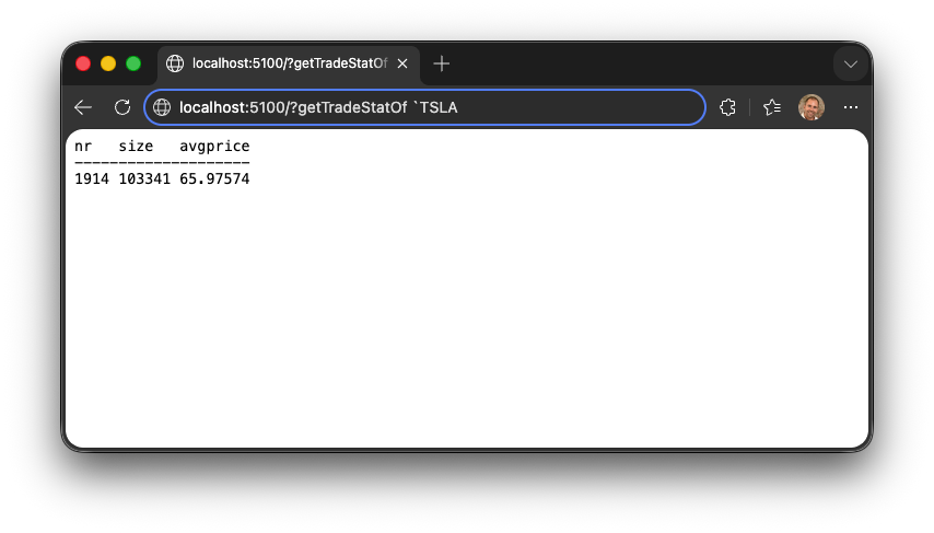
q)h (`getTradeStatOf; `TSLA)    / Simpler and safer than string manipulation
nr   size   avgprice
--------------------
1914 103341 65.97574
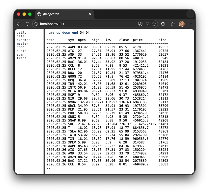
Connect from a web browser
Every q process started with -p is also a lightweight web server. This is incredibly useful for quick inspections. If you navigate to http://localhost:5100 in your browser, you can see all the variables currently in memory. Click on a variable to see its content.
You can even execute queries directly from the URL bar by appending a ? followed by your q code:
The advantage of a unified architecture
Traditional enterprise architectures suffer from "impedance mismatch." In these systems, data is stored in a relational database while business logic is written in a separate application layer using languages like Java, Rust, or Python. This separation creates significant friction: a substantial amount of engineering resources is wasted on Object-Relational Mapping (ORM) and data serialization — simply translating data from database rows into programming objects. Furthermore, to improve performance, developers often split logic between the two layers using brittle stored procedures, creating a fragile environment that is difficult to synchronize, test, and maintain.
KDB-X eliminates this overhead by providing a unified framework. In the q ecosystem, there is no distinction between the database and the programming language; the table is a native data structure. Business logic lives directly alongside the data, allowing for complex calculations to be executed where the data resides rather than moving massive datasets across a network to an application server. This proximity ensures that data traversal is minimized, resulting in performance gains that would be impossible in a multi-tier architecture.
This architectural simplicity translates into a significantly lower Total Cost of Ownership (TCO) for organizations. By collapsing the stack into a single layer, organizations reduce their hardware footprint and simplify their deployment pipelines. Maintenance becomes more straightforward because there is a single environment for both data and logic. Ultimately, this allows smaller teams of "dev-analysts" to build and support systems that would typically require large, specialized departments in a traditional software stack.
From language to architecture: kdb+ tick
Everything described so far – the vector engine, columnar tables, q-sql, memory-mapped partitions, and the database server – forms the q programming language and its runtime. But q is not just a tool for analysts; it is a platform for building production‑grade systems. The canonical example is kdb+ tick, the most widely used architecture ever implemented in q.
Released in the early 2000s, kdb+ tick is a complete, production-grade streaming data architecture for capturing, storing, and querying high-frequency time-series data in real time. Its most remarkable feature is its size: the entire system is implemented in just 34 lines of q code. There is no boilerplate and no scaffolding – only the essential logic required to ingest and publish real‑time data.
Despite its brevity, kdb+ tick has been deployed at the majority of the world's leading investment banks and financial institutions for over two decades. It processes billions of financial events – trades, quotes, order book updates – every single trading day, making it one of the most battle-tested real-time data systems ever built for electronic trading.
Three processes, one architecture
kdb+ tick separates responsibility across three specialized q processes, each optimized for a specific function.
- The Tickerplant (TP) is a low-latency, high-volume publish-subscribe hub that decouples data publishers from their subscribers.
- The Real-Time Database (RDB) subscribes to the tickerplant and collects today's data entirely in memory. New records become queryable within milliseconds, and the columnar in-memory layout enables complex analytical queries over millions of intraday rows to execute in microseconds.
- The Historical Database (HDB) stores all previous days' data using the splayed, partitioned layout described earlier in the persistence section. It memory-maps this data rather than loading it into RAM, allowing the system to address petabytes of historical time-series while reading only the columns and partitions required for a query.
The architecture addresses failure scenarios. For example, if the RDB process exits unexpectedly – because of hardware faults, operating‑system signals, or unbounded queries – it automatically recovers on restart.
The HDB scales horizontally to support hundreds of concurrent users through TCP socket sharding, a technique built into the q runtime. Because q's memory-mapped data is inherently read-only and shared across threads, the system requires no locking and performs no data copying. Increasing capacity is purely a configuration change, not a code change.
kdb+ tick is the clearest demonstration of what the q ecosystem was designed to enable. The language is not just a query tool bolted onto a database; it is a substrate from which entire systems can be composed. The 34 lines of code that implement kdb+ tick have processed more financial data than almost any other software system ever written, precisely because q eliminates everything that does not directly contribute to solving the problem at hand.
Next steps
- Read Q for Mortals if you prefer a book‑style introduction with more detail.
- Explore other tutorials to continue your learning journey.