3. Lists
3.0 Overview
All data structures in q are ultimately built from lists: a dictionary is a pair of lists; a table is a special dictionary; a keyed table is a pair of tables. Thus it is important to have a thorough grounding in lists.
All lists are equal but some lists are more equal than others. These are the lists of atoms of homogeneous type, called simple lists - known in mathematics as vectors. They have optimum storage and performance characteristics.
While q's list operations are similar to those in other functional languages, lists are stored and processed quite differently.
- They are not stored as linked lists under the covers. Simple lists occupy contiguous storage and general lists are pointers in contiguous storage.
- They grow by appending items to the end rather than "cons"-ing to the front.
- Efficient direct item access is available via indexing.
- A general list can hold items of different type without resorting to a union
sumtype to uniformize them.
It is instructive to think of q lists as dynamically allocated arrays.
3.1 Introduction to Lists
A list is an ordered collection. "A collection of what?" you ask. More precisely, a list is inductively defined as an ordered collection of atoms and other lists. We pay special attention to the case in which the list comprises atoms of uniform type.
3.1.1 List Definition and Assignment
A (general) list is an ordered collection of q data. The members of the collection are its items. The notation for the specification of a general list (list definition syntax) encloses values separated by semicolons within matching parentheses. Here is the format for creating a list literal with n items.
(v0;v1; … ;vn-1)
Tip
Whitespace after the separators in list definition is optional. In what follows, we shall often insert optional whitespace after the semicolon separators for readability. This is a personal style that you may choose not to follow.
Following are examples of literal list definitions and their resulting console displays.
q)(1; 1.1; `1)
1
1.1
`1
q)(1;2;3)
1 2 3
q)("a";"b";"c";"d")
"abcd"
q)(`Life;`the;`Universe;`and;`Everything)
Life`the`Universe`and`Everything
q)(-10.0; 3.1415e; 1b; `abc; "z")
-10f
3.1415e
1b
`abc
"z"
q)((1; 2; 3); (4; 5))
1 2 3
4 5
q)((1; 2; 3); (`1; "2"; 3); 4.4)
1 2 3
(`1;"2";3)
4.4
If you diligently entered each of these examples in your console, you have noticed that q does not always echo what you type. The initial and last three lists are general lists, meaning they are not homogeneous atoms. This could mean atoms of mixed type, nested lists of uniform type, or atoms and/or nested lists of mixed type.
Items in a list are sequenced left-to-right via the ;, providing an inherent order.
q)n:1
q)(n; n+1; n+2)
1 2 3
In particular, the lists (1;2) and (2;1) are different. SQL is based on sets, which are inherently unordered. This distinction leads to some subtle differences between the semantics of queries on q tables versus the analogous SQL queries. The inherent ordering of lists makes large time series processing natural and fast in q, while it is cumbersome and slow in standard SQL due to the need to place things in order when they are retrieved.
Lists can be assigned to variables exactly like atoms.
q)L1:(1; 2; 3)
q)L2:("z";"a";"p";"h";"o";"d")
q)L3:((1; 2; 3); (`1; "2"; 3); 4.4)
Advanced
For those who already know some q, we point out that literal list definition is just syntactic sugar for the multivalent function enlist. Thus if items are omitted in a literal list definition, the result is a projection of the associated enlist whose omitted parameters capture values for the empty slots.
q)type (1;;3) / is actually enlist[1;;3]
104h
q)(1;;3) 2
1 2 3
q)f:(1;;3)
q)f 2
1 2 3
q)f:(1;;) / is actually enlist[1;;]
q)f[2;3]
1 2 3
3.1.2 count
The number of items in a list is its count. You obtain the count of a list by asking for it.
q)count (1; 2; 3)
3
q)count L1
3
This is our first direct encounter with a q function (also called an operator in some contexts), which we will learn about in Chapters 4 and 6. For now, we need only understand that count returns an integer equal to the number of items in the list that follows it.
Tip
The maximum number of items for a list is 264-1.
Observe that the count of an atom is 1.
q)count 42
1
q)count `zaphod
1
3.2 Simple Lists
A list of atoms of a uniform type, called a simple list, corresponds to the mathematical notion of a vector. Such lists are treated specially in q. They have a simplified notation, take less storage and compute faster than general lists.
Tip
You can always enter lists in general list notation, even for simple lists.
Whenever q recognizes that the items of a list are homogeneous atoms, it dynamically converts to a simple list without asking for permission. It most cases, the storage and performance advantages justify the imposition. However, in some cases – such as deletion of an outlier item of non-uniform type – this causes a programming headache because the list will no longer allow appends or updates with items that do not conform to the resulting uniform type.
3.2.1 Simple Integer Lists
The console display of a simple list of any numeric type omits the enclosing parentheses and replaces the separating semicolons with (required) blanks. The following two expressions define the same list, as q verifies by testing for identity using ~.
q)(100;200;300)
100 200 300
q)100 200 300
100 200 300
q)100 200 300~(100; 200 ; 300)
1b
The console display of the first expression demonstrates the automatic conversion to simple lists previously mentioned.
Similar notation, with the addition of a single trailing type indicator, is used for simple lists of short and int.
q)(1h; 2h; 3h)
1 2 3h
q)(100i; 200i; 300i)
100 200 300i
Tip
The trailing type indicator in the console display applies to the entire list and not just the last item of the list; otherwise, the list would not be simple and would be displayed in general form.
q)(1; 2; 3h)
1
2
3h
3.2.2 Simple Floating Point Lists
Simple lists of float and real are notated the same as integers.
q)(123.4567; 9876.543; 99.0)
123.4567 9876.543 99
q)123.4567 9876.543 99
123.4567 9876.543 99
Observe that the q console suppresses the decimal point when displaying a float having zero(es) to the right of the decimal; but the value is not an integer. This notational efficiency for float display means that a list of floats having no decimal parts displays with a trailing f.
q)1.0 2.0 3.0
1 2 3f
q)1 2 3f~1.0 2.0 3.0
1b
Also observe that if you include what appears to be an integer in a list of float, q assumes that you are following its convention and merely omitting redundant data to the right of the decimal. That is, you get a list of float and not a general list.
q)1.1 2 3.3~1.1 2.0 3.3
1b
3.2.3 Simple Binary Lists
The abbreviated notation for a simple list of boolean or byte data juxtaposes the individual data values together with a type indicator. The 'b' type indicator for boolean trails the list.
q)(0b;1b;0b;1b;1b)
01011b
q)01011b
01011b
The '0x' indicator for byte precedes the list.
q)(0x20;0xa1;0xff)
0x20a1ff
q)0x20a1ff~(0x20;0xa1;0xff)
1b
Tip
A simple list of boolean atoms requires the same number of bytes to store as it has atoms. While the simplified notation is suggestive of a bit mask, multiple bits are not compressed to fit inside a single byte. The boolean list above uses 5 bytes of storage.
The display of a simple list of GUIDs is the same as that of integers - i.e., the values are separated by spaces.
q)2?0Ng
ddb87915-b672-2c32-a6cf-296061671e9d 580d8c87-e557-0db1-3a19-cb3a44d623b1
3.2.4 Simple Symbol Lists
The abbreviated notation for simple lists of symbols juxtaposes the individual atoms with no intervening whitespace.
q)(`Life;`the;`Universe;`and;`Everything)
`Life`the`Universe`and`Everything
Inserting spaces between symbol atoms causes an error.
q)`bad `news
'bad
 [0] `bad `news
    ^
3.2.5 Simple char Lists and Strings
The simplified notation for a list of char looks just like a string in most languages, with the juxtaposed sequence of characters enclosed in double quotes.
q)("s"; "t"; "r"; "i"; "n"; "g")
"string"
q)"string"~("s"; "t"; "r"; "i"; "n"; "g")
1b
A simple list of char is called a string; however, it does not have the semantics of a string in most languages. Since it is a list of char, not an atom, you cannot ask if two strings of different lengths are equal. You can ask if they are identical (as you can with any two q entities).
q)"string"="text"
'length
q)"string"~"text"
0b
3.2.6 Lists of Temporal Data
Since they are really integers under the covers, the abbreviated form for simple temporal lists separates items with a space.
q)(2000.01.01; 2001.01.01; 2002.01.01)
2000.01.01 2001.01.01 2002.01.01
q)(00:00:00.000; 00:00:01.000; 00:00:02.000)
00:00:00.000 00:00:01.000 00:00:02.000
Specifying a list of mixed temporal types has a different behavior from that of a list of mixed numeric types. In this case, the list takes the type of the widest item in the list; other items are widened.
q)12:34 01:02:03
12:34:00 01:02:03
q)01:02:03 12:34
01:02:03 12:34:00
To force the type of a mixed list of temporal values, append a type specifier.
q)01:02:03 12:34 11:59:59.999u
01:02 12:34 11:59
3.3 Empty and Singleton Lists
Lists with one or no items merit special consideration, especially since q's notation and display are not exactly friendly.
3.3.1 The General Empty List
It is useful to have lists with no items. A pair of parentheses enclosing nothing (except optional whitespace) denotes the general empty list, which (annoyingly) has no console display.
q)()
q)
We shall see in 6.2 that it is possible to define an empty list with a specific type, so that it becomes a list with 0 items of that type. This is used to force type checking for items that are appended to the list.
Advanced
If you want to force the display of an empty list, use the q utility .Q.s1, which converts any q entity into a string suitable for display.
q)L:()
q)L
q)-3!L
"()"
3.3.2 Singleton Lists
A singleton is a list containing a single item. As any postal clerk will tell you, an item in a box is not the same as an unboxed item. So an atom and a singleton containing that atom are different.
The syntax of a singleton presents a notational conundrum for q. We might expect to write the singleton list containing 42 as (42) but we cannot. The issue arises from q's use of parentheses both for literal list syntax and for the usual mathematical grouping in expressions. The latter leads to the following sequence of arithmetic reductions.
(40+2) 🡪 (42) 🡪 42
This forces (42) to be the atom 42.
Unfortunately, there is no way to type a singleton literal. Singletons are created by the function enlist, which manages to avoid the usual q predilection for aggressively short names.
q)enlist 42
,42
Observe that the console display of a singleton list uses the k form of enlist - i.e., unary ,. Don't be fooled: we can't use this in q.
q),42
',
[0] ,42
    ^
Tip
A string with a single character cannot be written syntactically as "a" - this is a character atom. Use enlist. This is
a common error for qbies, especially with writing lists of strings.
q)"a"
"a"
q)enlist "a"
,"a"
A singleton need not contain an atom as its sole item; it can be any q entity.
q)enlist 1 2 3
1 2 3
q)enlist (10 20 30; `a`b`c)
10 20 30 a b c
3.4 Indexing
A list is sequenced from left-to-right in the position of its items. The offset of an item from the beginning of the list is called its index. The initial item has index 0, the second item has index 1, etc. Thus a list of count n has items at indices 0 through n - 1.
Tip
There is no item at index n. This is a common newbie mistake.
3.4.1 Index Notation
To access the item at index i in a list, follow the list with [i]. This is called item indexing. For example,
q)(100; 200; 300)[0]
100
q)100 200 300[0]
100
q)L:100 200 300
q)L[0]
100
q)L[1]
200
q)L[3] / index out of bounds
0N
q)L[2]
300
3.4.2 Indexed Assignment
Items in a list can also be assigned via item indexing. Thus,
q)L:1 2 3
q)L[1]:42
q)L
1 42 3
Important
Index assignment into a simple list enforces strict type matching with no type promotion. Otherwise put, when you assign an item in a simple list, the type must match exactly and a narrower type is not widened.
q)L:100 200 300
q)L[1]:42h
'type
This may come as a surprise if you are accustomed to numeric values always being promoted to wider types in dynamically typed languages – e.g., q itself.
Tip
Should you find exceptions to this in earlier releases of q, do not count on them being in future releases!
3.4.3 Indexing Domain
Providing an non-integral data type for the index results in an error.
q)L:(-10.0; 3.1415e; 1b; `abc; "z")
q)L[1.0]
'type
In contrast, if you index outside the proper bounds of the list, the result is not an error. Instead you get a null value indicating "missing data." Specifically, indexing outside the range of 0 to (count L) – 1 yields a null of the type of the item at index 0. This is the most efficient thing to return in the case of a general list where there is no canonical type.
q)L1:1 2 3 4
q)L1[4]
0N
q)L2:1.1 2.2 3.3
q)L2[-1]
0n
q)L3:(`1; 2; 3.3)
q)L3[0W]
`
Tip
Pay special attention to the first example above that indexes the list at its count. Indexing one position past the end of the list is easy for qbies if you’re not used to indexing relative to 0.
3.4.4 Empty Index and Null Item
An omitted index returns the entire list.
q)L:10 20 30 40
q)L[]
10 20 30 40
An omitted index is not the same as indexing with an empty list. The latter returns an empty list, so we use the .Q.s1 utility to reveal its display.
q).Q.s1 L[()]
"()"
The syntactic form double-colon :: denotes a missing item in the context of an index, which allows explicit notation or programmatic generation of an empty index.
q)L[::]
10 20 30 40
Note
When used in this way the token :: standards for missing data - i.e., it is a null. The type of :: does not match "normal" data types in q so that it can effectively be used as a null in most contexts. The KX Documentation refers to it as the "general null". We find that verbose and in this tutorial we will stick to calling it nil when used in this context.
q)L:(::; 1 ; 2 ; 3)
q)type L
0h
q).Q.s1 L[0]
"::"
This is one way to avoid a nasty surprise when q would otherwise automatically convert a list to simple type. A simple case is when you reassign the only non-conforming item in the list.
q)L:(1; 2; 3; `a)
q)L[3]:4
q)L
1 2 3 4
q)L[3]:`a
"type
After the assignment you can no longer re-assign `a back into the list in its original position. One way to avoid this by placing :: in the list as a guard.
q)L:(::; 1 ; 2 ; 3; `a)
q)L[4]:4
q)L[4]:`a
q)
One caution for this technique is that you must avoid passing :: on to expressions that use the actual data in the list.
3.4.5 Lists with Expressions
Any valid q expression can occur in list definition.
q)a:42
q)b:43
q)(a; b)
42 43
q)L1:1 2 3
q)L2:40 50
q)(L1; L2)
1 2 3
40 50
q)(count L1; sum L2)
3 90
Tip
You cannot use the abbreviated notation of simple lists with variables.
q)a:42
q)b:43
q)a b
'Cannot write to handle 42. OS reports: Bad file descriptor
The reason for this cryptic error message will be apparent when we deal with files later.
3.5 Combining Lists
3.5.1 Joining with ,
We scoop the presentation on operators in the next chapter to describe a few list operators used frequently with lists. First is the join operator ,. Its result is a new list in which (a copy of) the right operand is appended to the end of (a copy of) the left operand. Join accepts an atom in either argument - i.e., as if the corresponding singleton had been supplied.
q)1 2 3,4 5
1 2 3 4 5
q)1,2 3 4
1 2 3 4
q)1 2 3,4
1 2 3 4
Observe that if the arguments are not of uniform type, the result is a general list.
q)1 2 3,4.4 5.5
1
2
3
4.4
5.5
Tip
To ensure that a q entity x becomes a list, use either (),x or x,(). This leaves a list unchanged but effectively enlists an atom. Such a seemingly trivial expression is actually useful and is our first example of a q idiom. You cannot use enlist x for the same purpose. Why not?
3.5.2 Merging with (^)
One way to combine two lists of the same length is by coalescing them with ^. The result is given by the rule that the right item prevails over the corresponding left item except when the right item is null, in which case the left item prevails.
q)L1:10 0N 30
q)L2:100 200 0N
q)L1^L2
100 200 30
3.6 Lists as Maps
Thus far, we have considered a list as data - i.e., a static collection of its items. We can also view it as a mathematical mapping provided by item indexing. Specifically, a list provides a map whose domain is integers and whose codomain is the collection of its items (supplemented with a null value). The list map assigns the output value L[i] to the input value i.
i |---> L[i]
Here are the I/O tables for some basic lists
101 102 103 104
| I | O |
|---|---|
| 0 | 101 |
| 1 | 102 |
| 2 | 103 |
| 3 | 104 |
(`a; 123.45; 1b)
| I | O |
|---|---|
| 0 | `a |
| 1 | 123.45 |
| 2 | 1b |
(1 2; 3 4)
| I | O |
|---|---|
| 0 | 1 2 |
| 1 | 3 4 |
The codomains of the first two examples are both collections of atoms. The last example has a codomain comprising lists.
A list not only acts like a map, it is a unary map whose notation is the same as function application. This is a useful way of looking at things. We shall see in Chapter 4 that a nested list can be viewed as a multivalent map.
From the perspective of lists as maps, the fact that indexing outside the bounds of a list returns a null means the map is implicitly extended to the domain of all integers with null output value outside the list proper.
3.7 Nesting
Data complexity can be built by using lists as items of lists.
3.7.1 Depth
Now that we're comfortable with simple lists, we return to general lists. Nested lists have item(s) that are themselves lists. The number of levels of nesting for a list is called its depth. Informally, the depth measures how much repeated indexing is necessary to arrive at only atoms. Atoms have depth 0 and simple lists have depth 1.
The notation of complex lists is reflected in nested parentheses. For pedagogical purposes, in this section only, we shall often use general notation to define even simple lists since the parentheses make things manifest. However, the console always displays lists in a concise form.
Following is a list of depth 2 that has three items, the first two being atoms and the last a list. We also show its simplified notation.
q)L:(1;2;(100;200))
q)count L
3
q)L:(1;2;100 200)
q3
q)L[0]
1
q)L[1]
2
q)L[2]
100 200
3.7.2 Pictorial Representation
We present a pictorial representation that may help in visualizing levels of nesting. An atom is represented as a circle containing its value. A list is represented as a box containing its items. A general list is a box containing boxes and atoms.
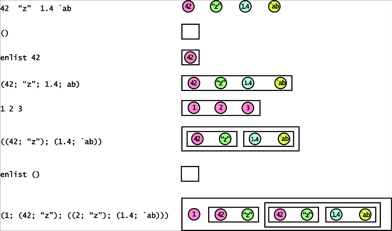
3.7.3 Examples
Following is a list of depth 2 with two elements, each of which is a simple list.
q)L2:((1;2;3);(`ab;`c))
q)count L2
2
Following is a list of depth 2 having three elements, two of which are general lists and one is an atom.
q)L3:((1; 2h; 3j); ("a"; `bc`de); 1.23)
q)count L3
3
q)L3[1]
"a"
`bcd
q)count L3[1]
2
Following is a list of depth 2 having one item that is a simple list.
q)L4:enlist 1 2 3 4
q)count L4
1
q)count L4[0]
4
Following is a "rectangular" list that can be thought of as the 3x4 matrix its display resembles.
q)m:((11; 12; 13; 14); (21; 22; 23; 24); (31; 32; 33; 34))
q)m
11 12 13 14
21 22 23 24
31 32 33 34
q)m[0]
11 12 13 14
q)m[1]
21 22 23 24
q)m[1][0]
21
3.8 Iterated Indexing and Indexing at Depth
In the examples above, we saw that the display of nested lists suggests arrays from other languages. You can indeed think of them as "ragged" arrays, provided you are careful about the iterated indexing. Indexing at depth is an alternative notation that suggests nested lists can also be viewed as higher dimensional arrays.
3.8.1 Iterated Item Indexing
Retrieving an item in a nested list via a single index retrieves a top-most item.
q)L:(1; (100; 200; (1000; 2000; 3000; 4000)))
q)L[0]
1
q)L[1]
100
200
1000 2000 3000 4000
Interpreting list indexing as function application for positional retrieval, we can read the last line in normal left-to-right fashion as,
From L retrieve the item at index 1
Since the result L[1] is itself a list, we can also retrieve its items via indexing. For example,
q)L[1][2]
1000 2000 3000 4000
Read this as,
From the item in L at index 1 retrieve the item at index 2
We can once again index into this result.
q)L[1][2][0]
1000
Read this as,
From the item in L at index 1 retrieve the item at index 2 and from this retrieve the item at index 0
3.8.2 Indexing at Depth
There is an alternative notation for iterated indexing into a nested list. It is strictly syntactic sugar and amounts to the same thing under the covers. This notation is called indexing at depth and it looks exactly like application of a multivalent function (which, in fact, it is). The previous retrieval can also be written as,
q)L[1;2;0]
1000
To summarize: indexing at depth simplifies the notation for retrieval of inner items from a nested list.
Tip
The semicolons in indexing at depth notation might make it appear that the collection of indices is a list. It is not, although we shall see later a way to perform indexing at depth in which the indices are a list. Also, don't confuse the semicolons with commas.
Assignment via index at depth works but assignment does not work with iterated indexing.
q)L:(1; (100; 200; (1000 2000 3000 4000)))
q)L[1; 2; 0]:999
q)L
1
(100;200;999 2000 3000 4000)
q)L[1][2][0]:42
'nyi
The last expression fails essentially because the intermediate retrievals have already been extracted and are not addressable.
To confirm that the notation for indexing at depth is reasonable, we return to our "matrix" example,
q)m:((11; 12; 13; 14); (21; 22; 23; 24); (31; 32; 33; 34))
q)m
11 12 13 14
21 22 23 24
31 32 33 34
q)m[0][0]
11
q)m[0][0]
11
q)m[0; 1]
12
q)m[1; 2]
23
The indexing at depth notation suggests thinking of m as a multi-dimensional matrix, whereas repeated single indexing suggests
thinking of it as an array of arrays. Chacun à son goût.
Advanced
It is possible to create a (ragged) array of a given number of rows or columns from a flat list using the reshape operator
# by specifying 0N (missing data) for the number of rows of column in the left operand.
q)2 0N#til 10
0 1 2 3 4
5 6 7 8 9
q)0N 3#til 10
0 1 2
3 4 5
6 7 8
,9
3.9 Indexing via Lists
As a vector language, q prefers to deal with lists whenever possible and so should you. There is no reason to restrict list retrieval to one item at a time. Indeed, we can ask for a list of items by passing a list of indices.
3.9.1 Retrieving Multiple Items
In this section, we begin to see the power of q as a vector language. We start with,
q)L:100 200 300 400
We know how to index single items of the list.
q)L[0]
100
q)L[2]
300
By extension, we can retrieve a list of multiple items via multiple indices. For simplicity we use simple list notation for the indices.
q)L[0 2]
100 300
The indices can be in any order, or even be duplicated and the corresponding items are retrieved. The shape of the output conforms to the input.
q)L[3 2 0 1]
400 300 100 200
q)L[0 2 0]
100 300 100
Here are some examples of indexing into literal lists.
q)01101011b[0 2 4]
011b
q)"beeblebrox"[0 7 8]
"bro"
Tip
Using a list as an index demonstrates that getting the semicolon separators right is essential when indexing at depth. Leaving them out or using commas effectively specifies multiple indices and you will get a corresponding list of values from the top level.
3.9.2 Indexing via a Variable
When retrieving items via multiple indices, the indices can live in a variable. Continuing with our previous example.
q)L
100 200 300 400
q)I:0 2
q)L[I]
100 300
3.9.3 Indexing with Nested Lists
Observe that in the examples of list indexing, the result of index retrieval has the same shape as the index. If the index is an atom the result is an atom. When the index list was a simple list, the result was a list of the same count.
More generally, we can retrieve via an arbitrary collection of indices. The retrieved list has the same shape as the index list.
q)L:100 200 300 400
q)L[(0 1; 2 3)]
100 200
300 400
Do not confuse this with indexing at depth. In the present case all items are retrieved at the top level only.
Advanced
More precisely, the result of indexing via a list conforms to the index list. The notion of conformability of lists is defined recursively. All atoms conform. Two lists conform if they have the same number of items and each of their corresponding items conform. In plain language, two lists conform if they have the same shape.
3.9.4 Assignment with List Indexing
Recall that a list item can be revised via item indexing,
q)L:100 200 300 400
q)L[0]:1000
q)L
1000 200 300 400
Assignment via index extends to indexing via a simple list with the proviso that the index list and value list conform.
q)L[1 2 3]:2000 3000 4000
q)L
1000 2000 3000 4000
Assignment via a simple index list is processed in sequence – i.e., from left-to-right. Thus,
q)L[3 2 1]:999 888 777
is equivalent to,
q)L[3]:999
q)L[2]:888
q)L[1]:777
Consequently, in the case of a repeated item in the index list (not a swell idea), the right-most assignment prevails.
q)L:100 200 300 400
q)L[0 1 0 3]:1000 2000 3000 4000
q)L
3000 2000 300 4000
You can assign a single value to multiple items in a list by using an atom for the assignment value. This is an example of a general phenomenon in q in which an atom is extended to conform to a list.
q)L:100 200 300 400
q)L[1 3]:999
q)L
100 999 300 999
3.9.5 Juxtaposition
Now that we’re familiar with retrieving and assigning via an index list, we introduce a simplified notation that is common in functional programming. It is permissible to leave out the brackets and juxtapose the list and index with separating whitespace (usually just a blank). Here are some examples.
q)L:100 200 300 400
q)L[0]
100
q)L 0
100
q)L[2 1]
300 200
q)L 2 1
300 200
q)I:2 1
q)L I
300 200
q)L ::
100 200 300 400
Which notation you use is a matter of personal preference. In this tutorial, we initially use brackets, since this notation is probably most comfortable for qbies coming from traditional programming. Experienced q programmers often use juxtaposition since it reduces notational density, although brackets can often eliminate parentheses.
3.9.6 Find ?
The Find operator is (and overload of) binary operator ? that returns the index of the first occurrence of the right operand in the left operand.
q)1001 1002 1003?1002
1
Tip
Since ? maps an item to its position, it is inverse to positional retrieval thought of as a function. In the case if duplicate items it isn’t quite an inverse.
If you try to find an item that is not in the list, the result is an integer equal to the count of the list.
q)1001 1002 1003?1004
3
One way to think of this result is that the position of an item that is not in the list is one past the end of the list, which is where it would be if you were to append it to the list.
Find is atomic in the right operand meaning that it extends to lists.
q)1001 1002 1003?1003 1001
2 0
3.10 Elided Indices
3.10.1 Eliding Indices for a Matrix
We return to the situation of indexing at depth for nested lists. For simplicity, we start with a rectangular list that displays as a matrix.
q)m:(1 2 3 4; 10 20 30 40; 100 200 300 400)
q)m
1 2 3 4
10 20 30 40
100 200 300 400
Analogy with traditional matrix notation suggests that we could retrieve a row or column from m by providing a “partial” index at depth. This indeed works because eliding an index in any slot is equivalent to specifying all legitimate indices for that slot.
q)m[1;]
10 20 30 40
q)m[;3]
4 40 400
Observe that eliding the last index reduces to item indexing at the top level.
q)m[1;]~m[1]
1b
Tip
Because of this correspondence, it is permissible to drop the trailing semicolon. We strongly recommend against this common practice as it makes code less obvious.
The situation of eliding the first index is more interesting. It essentially retrieves a "column" as a slice through the top-level lists - i.e., a row.
3.10.2 Eliding Indices for Deeply Nested Lists
Let's tackle three levels of nesting. Here we can elide one or two indices in any slot.
q)L:((1 2 3;4 5 6
7);(`a`b`c;`z`y`x`;`0`1`2);("now";"is";"the"))
q)L
(1 2 3;4 5 6 7)
(`a`b`c;`z`y`x`;`0`1`2)
("now";"is";"the")
q)L[;1;]
4 5 6 7
`z`y`x`
"is"
q)
q)L[;;2]
3 6
`c`x`2
"w e"
Interpret L[;1;] as,
Retrieve all items at index 1 of each top level list
Interpret L[;;2] as,
Retrieve the items at index 2 for each list at the second level
Observe that in L[;;2] the attempt to retrieve the item at index 2 of the string "is" was out of bounds and so resulted in the null char value " ". This is the source of the blank in "w e" of the result.
As the final exam for this section, let's combine an elided index with indexing by lists to retrieve a cross-section of L. Try to predict the result before entering the expression into your console session.
q)L[0 2;;0 1]
(1 2;4 5)
("no";"is";"th")
Interpret this as,
Retrieve the items at positions 0 and 1 from all columns in rows 0 and 2
Style recommendation
In general, it is permissible to elide all trailing semicolons arising from elided indices. We consider this bad practice. Looking at the notation below, would you guess that the expression after the comment was actually that to the left of it? We didn't think so.
L[1;;] / instead of L[1]
L[;1;] / instead of L[;1]
L[;;] / instead of L[]
3.11 Rectangular Lists and Matrices
3.11.1 Rectangular Lists
In this section, we further investigate matrix-like nested lists. A rectangular list is a list of lists all having the same count. Understand that this does not mean that a rectangular list is necessarily a traditional matrix, since there can be additional levels of nesting.
q)L:(1 2 3; (10 20; 100 200; 1000 2000))
q)L
1 2 3
10 20 100 200 1000 2000
A rectangular list can be transposed with flip, meaning that the rows and columns are reflected across the diagonal. When flip is applied to a rectangular list, it physically transposes the data - i.e., it allocates new storage and copies the original data in column order. This will not be the case for tables,
q)L:(1 2 3; 10 20 30; 100 200 300)
q)L
1 2 3
10 20 30
100 200 300
q)flip L
1 10 100
2 20 200
3 30 300
This effectively reverses the first and second slots in indexing at depth.
q)L:(1 2 3; 10 20 30; 100 200 300)
q)M:flip L
q)L[1;2]
30
q)M[2;1]
30
3.11.2 Formal Definition of Matrices
Matrices are a special case of rectangular lists and are defined recursively. A matrix of dimension 0 is a scalar. A matrix of dimension 1 is a simple list - i.e., a vector. The count of a vector is usually called its length or dimension in mathematics. Some functional programming languages have tuples, which can be thought of as coordinates of vectors with respect to a basis. Regrettably q does not.
In q, vectors do not need to be of numeric type.
q)v1:1 2 3. / vector of integers
q)v2:98.60 99.72 100.34 101.93 / float vector
q)v3:`so`long`and`thanks`for`all`the`fish / symbol vector
For n>1, we define a matrix of dimension n+1 as a list of matrices of dimension n all having the same size. Thus, a matrix of dimension 2 is a list of vectors, all having the same size. If all atoms in a matrix have the same type, we call this the type of the matrix.
3.11.3 Two and Three Dimensional Matrices
Let m be a two-dimensional matrix as defined in the previous section. The items of m are its rows. As we have already seen, the ith row of m can be obtained via item indexing as m[i]. Equivalently, we can use an elided index with indexing at depth to obtain the ith row as m[i;].
The console display of m in tabular form motivates defining the list m[;j] as the jth column of m. The notations m[i][j] and m[i;j] both retrieve the same item – namely, the item in row i and column j.
We make one final observation. Matrices are nested lists stored in row order. When the rows are simple, each occupies contiguous storage. This makes row retrieval very fast. On the other hand, columns must be picked out of the rows, so column operations are slower.
Advanced
By convention we consider a matrix to be a collection of rows. It would be equally valid to consider a two dimensional array as a collection of columns. As we shall see in Chapter 8, a table is a collection of columns that are logically (not physically) transposed for ease of indexing.
The constraints, retrieval and calculation of qSQL operate on columns, so they are fast, especially when the columns are simple lists. In particular, a simple time series can be represented by two parallel lists, one holding datetimes and the second holding the associated values.
Retrieving and manipulating the columns in vector operations is faster by orders of magnitude than performing the same operations in an RDBMS that stores data in rows with undefined order.
Higher dimensional matrices occur less frequently in q than in its ancestors. For completeness, here is an example of a three-dimensional 2x3x3 matrix - i.e., each of the two top-level items is a 3x3 matrix. While the console display of mm may appear to be unenlightening, it simply displays the items as a general list in row order.
q)mm:((1 2 3;4 5 6;7 8 9);(10 20 30; 40 50 60; 70 80 90))
q)mm
1 2 3 4 5 6 7 8 9
10 20 30 40 50 60 70 80 90
q)mm[0]
1 2 3
4 5 6
7 8 9
q)mm[1]
0 20 30
40 50 60
70 80 90
3.11.4 Matrix Flexibility*
We have seen that although there is no separate construct for matrices in q, rectangular lists look and act like their mathematical matrix counterparts. However, they have features not available in simple mathematical notation or in most traditional languages. We have seen that a rectangular list can be viewed and manipulated both as a multi-dimensional array (i.e., indexing at depth) and as an array of arrays (repeated item indexing). In addition, we can extend individual item indexing with indexing via lists.
q)m:(1 2; 10 20; 100 200; 1000 2000)
q)m 0 2
1 2
100 200
3.12 Pattern Matching on Lists (Advanced)
In its simplest form, List matching allows a q object to be compared against a template, matching its structure in order to assign variables to its parts, check types, and/or modify values. Effectively it inspects the object without vivisection. Introduced in q 4.1, it is powerful and can tidily encapsulate many steps in everyday coding. See 10.4 for the full treatment of pattern matching.
In this section we introduce a simple form, matching on assignment using list patterns. We present a sequence of increasingly involved examples, building our understanding of what a pattern can do at each step.
3.12.1 Pattern Matching on List Assignment
Pattern matching on assignment places a pattern template of the left hand sign of the assignment operator. It enhances the process of assignment to reach into the structure of the entity being assigned to access its constituent parts, which can be inspected, modified and assigned.
In the case of a list, the pattern template is a general list of special form and the constituent list items are themselves patterns. The syntax is new to q so it may take some practice to get it right. The pattern appears on the left hand side (lhs) of an assignment : and the list from which we will extract data appears on the right hand side (rhs). Here is our first example,
q)(x;y):(1;`nuba)
Note
Optional whitespace after separators can be used for readability.
Let’s break this down. In rhs we have a garden variety general list that is already in reduced form – i.e., any expressions have been evaluated. This list serves as the source of data to extract during the assignment.
Now examine lhs. We interpret this list as a pattern template that says: expect to receive a value for a variable x in the first slot and a value for a variable y in the second slot. Both are examples of the name pattern, meaning that the contents in that slot will be assigned to the variable named.
Note
If the variables x and y don’t already exist, they will be created in the assignment.
Now to the good stuff. When q sees an assignment with such a form of lhs and rhs, it requires the two lists to confirm exactly, so it first checks this. Remember that two lists conforming means they have the same shape/structure. A more precise definition is recursive, requiring the lists to have the same number of elements at each level of nesting.
In our case the lists do conform so q proceeds to the next step. It associates the variables in lhs with corresponding values in rhs and then performs assignments in the normal manner. As a result of the assignment we now have,
q)x
1
q)y
`nuba
The net effect is that we have assigned (different) values to x and y in a single assignment statement. This is something q programmers have desired for years.
Observe that the list containing x and y in lhs is actually created as well. In our case we ignored the value of the main assignment, but you can capture it.
q)z:(x;y):(1;`nuba)
q)z
1
`nuba
What happens if lhs and rhs don't conform? An error is raised and no assignments are performed. Continuing from before.
q)x,y
1
`nuba
q)r:(x;y):til 3
'length
[0] r:(x;y):til 3
^
q)x,y
1
`nuba
q)r
'r
Note that unlike most situations in q, an atom rhs is not extended to conform to a non-atom lhs.
q)(x;y):1
'type
 [0] (x;y):1
    ^
If rhs is not fully reduced, q first reduces it and then proceeds as before.
q)(x;y):(1+til 3; 2#"abc")
q)x
1 2 3
q)y
"ab"
If lhs is not fully reduced an error is raised
(x; y; 5*z):(1; `nuba; 10)
'nyi
 [0] (x; y; 5*z):(1; `nuba; 10)
    ^
Here is an example using a constant pattern, which verifies that a specific value is present but does not assign it.
q)(x;42):41 42
q)x
41
q)(x:42):42 43
'type
 [0]  (x:42):42 43
    ^
Here is a more complicated example showing that a pattern can assign variables at arbitrary levels of nesting.
q)(x;(10;y);(30;(300;z))):(1; (10 20); (30; 300 400))
q)x,y,z
1 20 400
Finally, an empty slot in lhs – i.e., an omitted item – results in a wildcard match with the corresponding item in rhs. The empty slot is an example of a null pattern which matches anything.
q)(1b;;x):(1b;`whatever;42 43)
q)x
42 43
This makes it easy to create a template targeted at only specific slots while ensuring the others are present. Take a typical instance of a list, place variables where you want things to be captured and then zap all the other values in the structure. For example, here is a pattern that matches a list of length 4 having value 3 at index 2 and that captures the last item in a variable something.
q)(;;3;something):(1;2;3;4)
q)something
4
3.12.2 Type Checking with Patterns
The next level of pattern matching is the type check pattern which performs type checking via inclusion of type chars in the form p:`x.
Advanced
The syntax is similar to table definition syntax whose basic form we recall – see 8.1.3 for a full explanation.
([] c:expr; …)
Here the : is not assignment; rather it is a marker to separate a column identifier to its left and an expression for the value of that column to its right. Under the covers q creates a symbolic column name, evaluates the expression and then includes both in a column dictionary that will eventually be flipped into the resulting table.
We start with the simplest example of a type check pattern.
(cat:`s)
First we point out the parentheses are required here and they are not list delimiters. In direct analogy with table definition, the : is not assignment. It is a marker that indicates an intended variable to its left. To its right is a symbol containing a q type char. Yeah that sounds a bit funky but you'll get over it. Now we can interpret our example pattern as: a variable cat is expecting to receive a value of type symbol.
Now the magic happens. We place this pattern on the left hand side (lhs) of an assignment. As before, q checks that the right hand side (rhs) and lhs conform. In this case they do since they are both atoms. Next, in preparation for performing the assignment, q checks that the type of the rhs value matches the corresponding type in the lhs. In our example the type matches so the assignment is made.
q)(cat:`s):`nuba
q)cat
`nuba
Type checking is another feature q programmers have been requesting for years. Let's see how far it goes.
First we note that this syntax is a generalization of the following, which works in previous versions of q. In this case the enclosing parentheses on the left are simply ignored. In the new context this is the degenerate case of type checking where no type is specified and checked.
q)(cat):`devi
q)cat
`devi
Now we combine type checking with list assignment of the previous section.
q)(fname:`s; lname:`s; age:`j):(`jeffry; `borror; 21)
q)fname,lname,age
`jeffry
`borror
21
Observe that the types must match exactly; no type promotion will be performed (although in the next section we will see how to accommodate that).
q)(fname:`s; lname:`s; age:`j):(`jeffry; `borror; 21i)
'type
 [0] (fname:`s; lname:`s; age:`j):(`jeffry; `borror; 21i)
                    ^
You can intermix variable assignment with and without type checking.
q)(fname:`s; lname:`s; age):(`jeffry; `borror; 21.6)
q)type age
-9h
If you want to perform type checking without capturing values, omit the variable names. Yeah it looks funky but it's nothing outrageous for q. Don't confuse this use of ':' with that indicating return from a function which we will meet later.
q)(:`s; :`f):(`hot; 102.0)
q)(:`s; :`f):(`hot; 102)
'type
 [0] (:`s; :`f):(`hot; 102)
    ^
Observe that the decimal point is required for the float value in this situation due to no type promotion.
Advanced
In practice you could wrap this pattern in protected evaluation and trap the error to create a customized type checking routine.
3.13 Basic List Operators
In this section we demonstrate simple use cases for some list operations that are used in following chapters.
3.13.1 til
The unary til takes a non-negative integer n and returns a list of n consecutive natural numbers starting at 0. It is useful for constructing regular lists of integers.
q)til 10
0 1 2 3 4 5 6 7 8 9
q)1+til 10
1 2 3 4 5 6 7 8 9 10
q)2*til 10
0 2 4 6 8 10 12 14 16 18
q)1+2*til 10
1 3 5 7 9 11 13 15 17 19
q)-5+4*til 3
-5 -1 3
Tip
If your code includes constructs of the form function each til count, you are almost certainly writing loopy – i.e., non-vector – code, otherwise known as VBQ or PYQ.
3.13.2 distinct
The unary function distinct returns the unique items in its list argument, in order of first occurrence.
q)distinct 1 2 3 2 3 4 6 4 3 5 6
1 2 3 4 6 5
3.13.3 where
The basic form of where returns the indices of 1b in a boolean list – i.e., it reports where the ones are.
q)where 101010b
0 2 4
This is useful to operate at positions that have been identified by a predicate.
q)L:10 20 30 40 50
q)L[where L>20]:42
q)L
10 20 42 42 42
3.13.4 group
The unary function group takes a list and returns a dictionary in which each distinct item of the argument is mapped to the indices of its occurrences, in order of occurrence.
q)group "i miss mississippi"
i| 0 3 8 11 14 17
| 1 6
m| 2 7
s| 4 5 9 10 12 13
p| 15 16