Apply predictive analytics to improve operations and reduce risks in manufacturing
For manufacturers, machine downtime can cost millions of dollars a year in lost profits, repair costs, and lost production time for employees. By embedding predictive analytics in applications, manufacturing managers can monitor the condition and performance of assets and predict failures before they happen.
The kdb Insights Enterprise exists to be the premier cloud-native platform for actionable, data-driven insights. The majority of data science efforts are spent wrangling data beforehand to build machine learning models and data visualizations to extract insights.
In this recipe you will apply compute logic to live data streaming in from the popular message service MQTT as well as use Deep Neural Network Regression to determine the likelihood of breakdowns.

Benefits
| Predictive analysis | Use predictive analytics and data visualizations to forecast a view of asset health and reliability performance. |
| Reduce risks | Leverage data in real time for detection of issues with processes and equipment, reducing costs and maximizing efficiencies throughout the supply chain with less overhead and risk. | Control logic | Explore how to rapidly develop and visualize computations to extract insights from live streaming data. |
Pre-requisites
Before you begin, you need access to a running instance of kdb Insights Enterprise.
Step 1: Build database
The goal of this step is to teach you how to build a database to store the data you need to ingest.
-
Select
Build a databasefrom the home screenGetting Startedpage.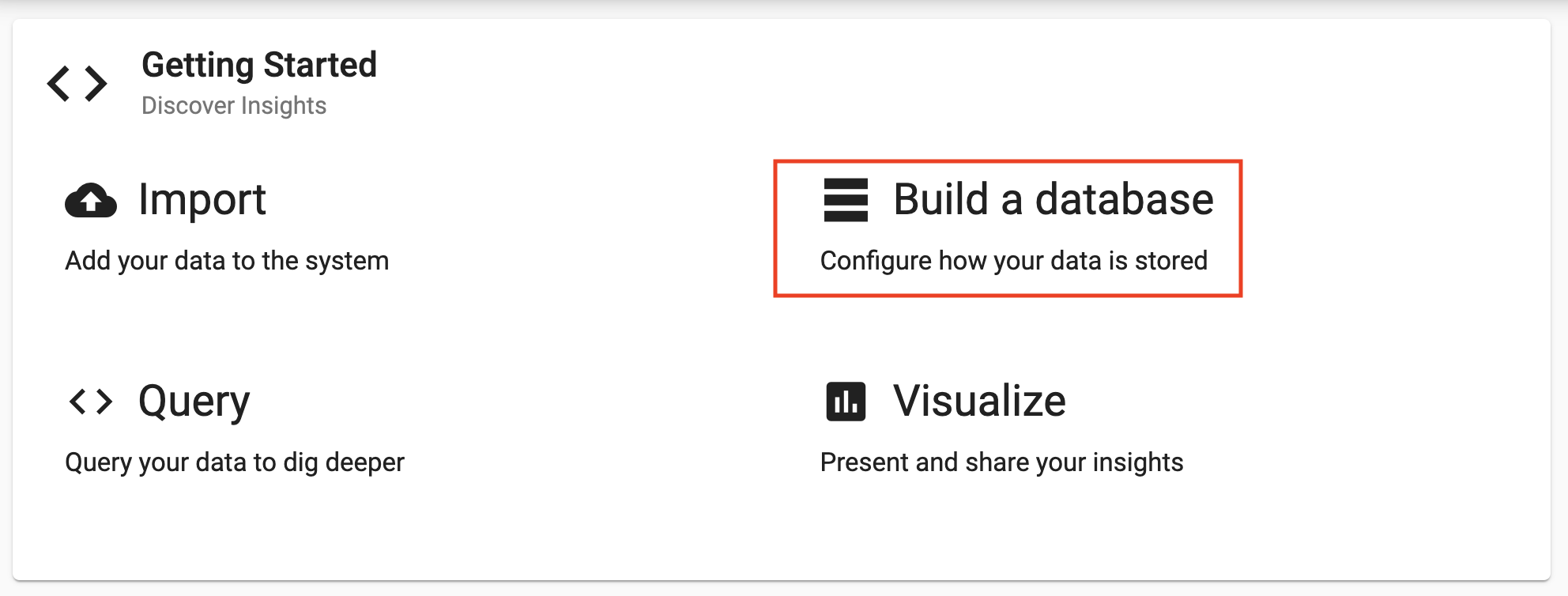
-
Enter the name and desired size of your database and then select
Next.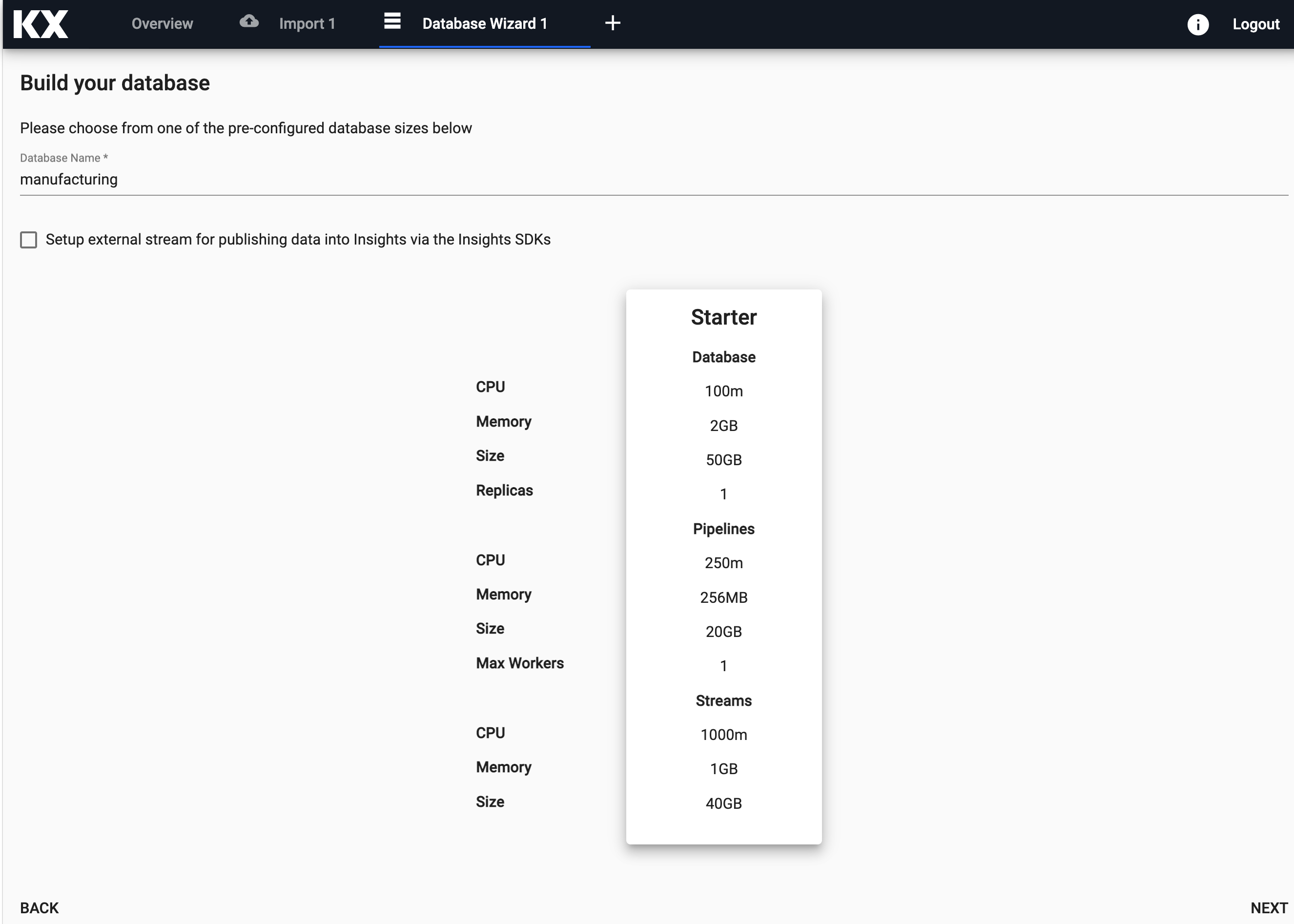
-
Select
Nextagain from the schema page.You do not need to enter any schema details on this page as you replace this default schema with one created in the upcoming steps 5-6.
-
Select
Save.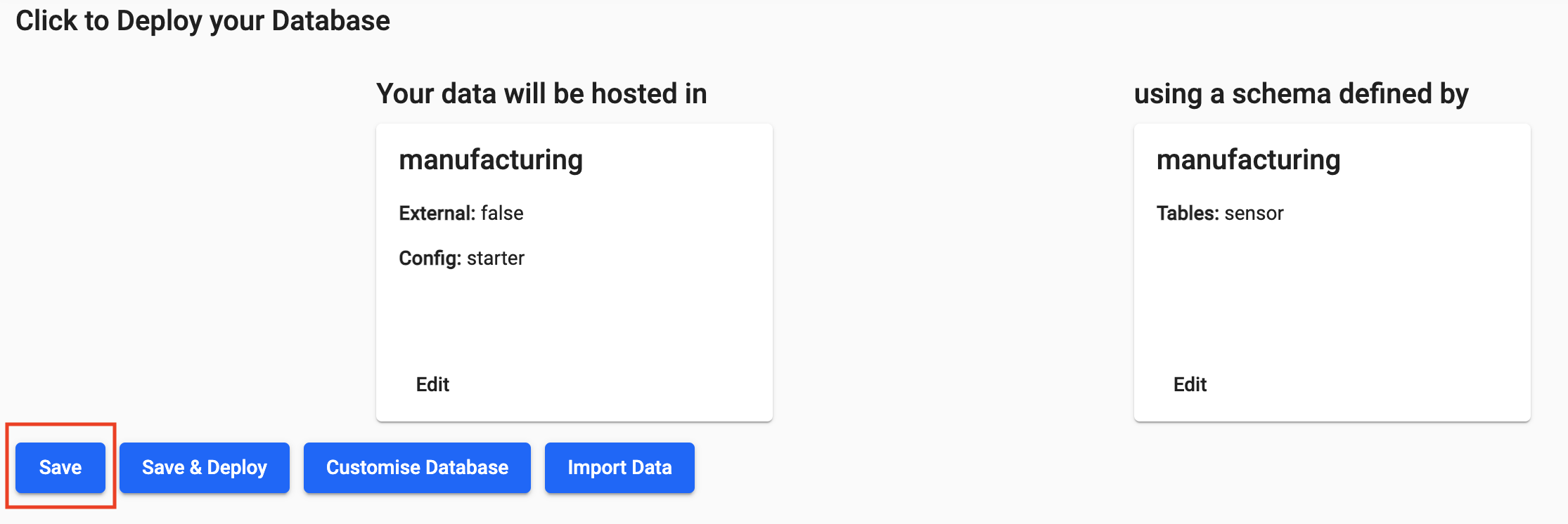 At this stage your database should look like this.
Do not deploy yet!
Do not deploy this assembly until you replace the schema with the custom one for this recipe.
-
Select the "+" icon from the toolbar at the top of the screen and then select
Schema.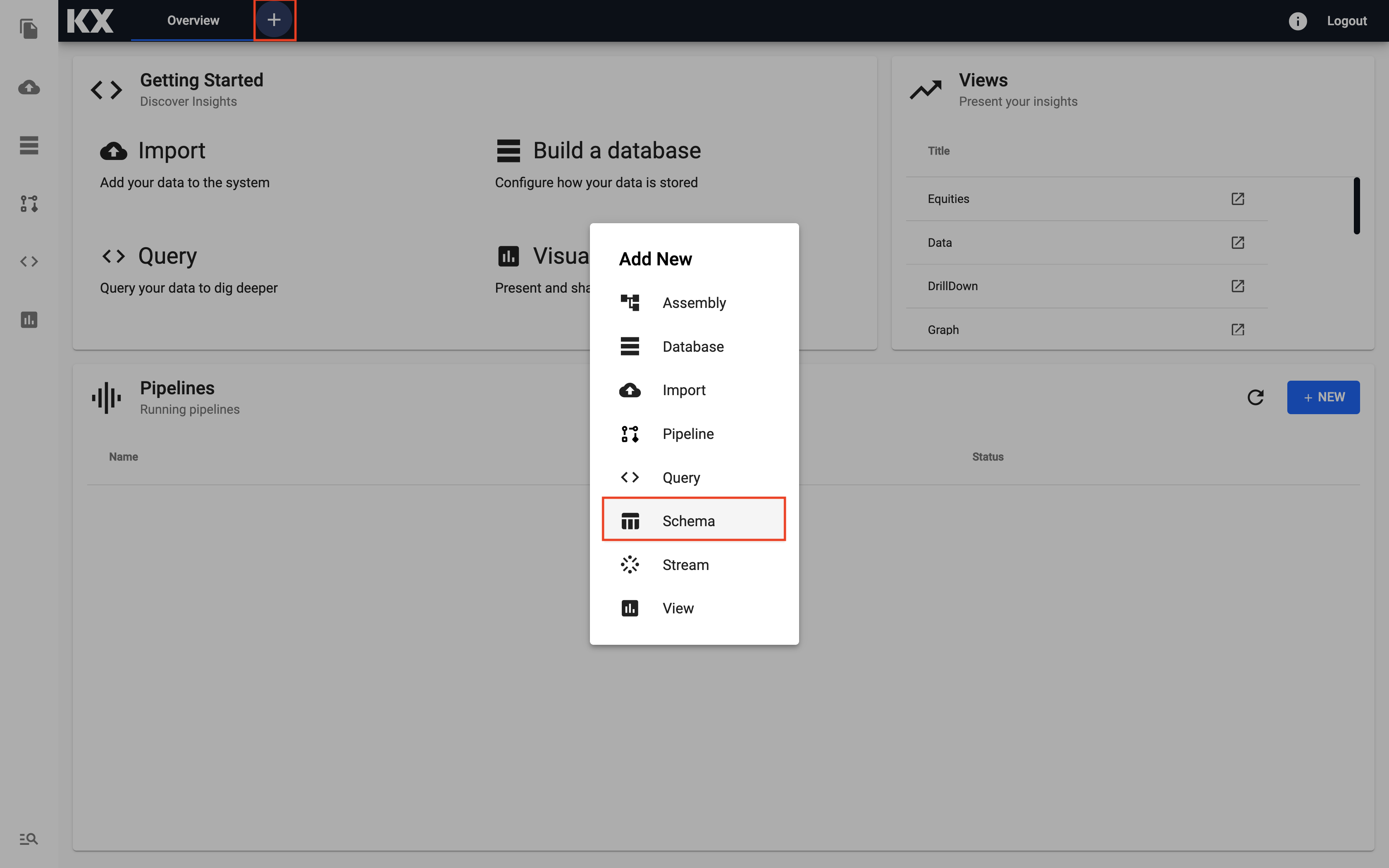
-
Name your schema.
Give the schema a new name
Do not give it the same name as the database created in the previous section as a default schema already exists with this name.
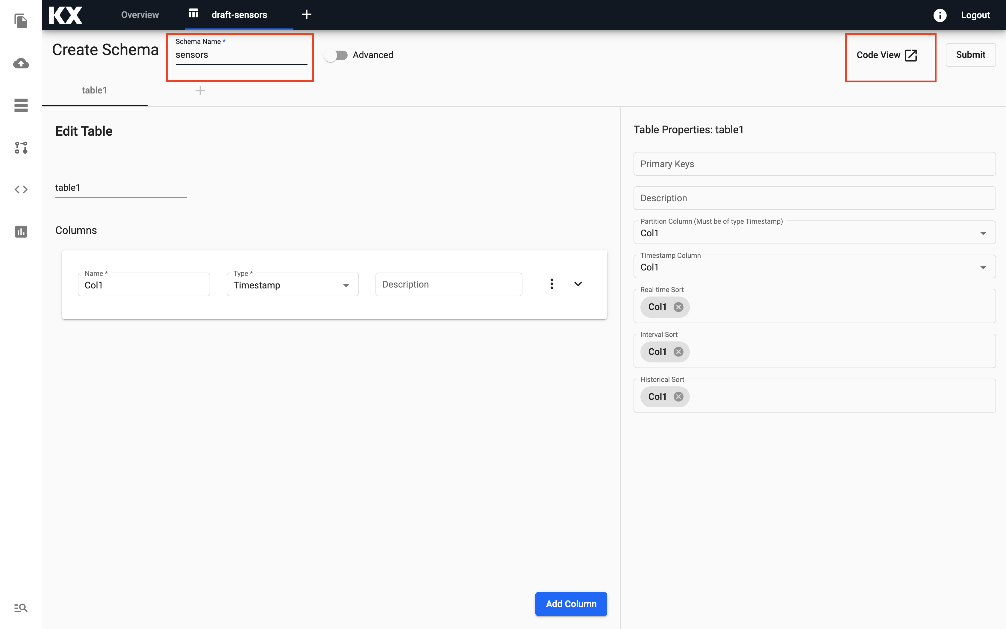
-
Select the
Code Viewbutton on the top right hand side and replace with the custom schema provided.Click to expand for schema!
Copy and paste these details into the Code View window and click Apply.[ { "name": "sensors", "type": "partitioned", "primaryKeys": [], "prtnCol": "time", "updTsCol": "time", "sortColsDisk": [ "time" ], "sortColsMem": [ "time" ], "sortColsOrd": [ "time" ], "columns": [ { "type": "timestamp", "attrDisk": "parted", "attrOrd": "parted", "name": "time", "primaryKey": false, "attrMem": "" }, { "name": "flowplant", "type": "float", "primaryKey": false, "attrMem": "", "attrOrd": "", "attrDisk": "" }, { "name": "pressplant", "type": "float", "primaryKey": false, "attrMem": "", "attrOrd": "", "attrDisk": "" }, { "name": "tempplantin", "type": "float", "primaryKey": false, "attrMem": "", "attrOrd": "", "attrDisk": "" }, { "name": "tempplantout", "type": "float", "primaryKey": false, "attrMem": "", "attrOrd": "", "attrDisk": "" }, { "name": "massprecryst", "type": "float", "primaryKey": false, "attrMem": "", "attrOrd": "", "attrDisk": "" }, { "name": "tempprecryst", "type": "float", "primaryKey": false, "attrMem": "", "attrOrd": "", "attrDisk": "" }, { "name": "masscryst1", "type": "float", "primaryKey": false, "attrMem": "", "attrOrd": "", "attrDisk": "" }, { "name": "masscryst2", "type": "float", "primaryKey": false, "attrMem": "", "attrOrd": "", "attrDisk": "" }, { "name": "masscryst3", "type": "float", "primaryKey": false, "attrMem": "", "attrOrd": "", "attrDisk": "" }, { "name": "masscryst4", "type": "float", "primaryKey": false, "attrMem": "", "attrOrd": "", "attrDisk": "" }, { "name": "masscryst5", "type": "float", "primaryKey": false, "attrMem": "", "attrOrd": "", "attrDisk": "" }, { "name": "tempcryst1", "type": "float", "primaryKey": false, "attrMem": "", "attrOrd": "", "attrDisk": "" }, { "name": "tempcryst2", "type": "float", "primaryKey": false, "attrMem": "", "attrOrd": "", "attrDisk": "" }, { "name": "tempcryst3", "type": "float", "primaryKey": false, "attrMem": "", "attrOrd": "", "attrDisk": "" }, { "name": "tempcryst4", "type": "float", "primaryKey": false, "attrMem": "", "attrOrd": "", "attrDisk": "" }, { "name": "tempcryst5", "type": "float", "primaryKey": false, "attrMem": "", "attrOrd": "", "attrDisk": "" }, { "name": "temploop1", "type": "float", "primaryKey": false, "attrMem": "", "attrOrd": "", "attrDisk": "" }, { "name": "temploop2", "type": "float", "primaryKey": false, "attrMem": "", "attrOrd": "", "attrDisk": "" }, { "name": "temploop3", "type": "float", "primaryKey": false, "attrMem": "", "attrOrd": "", "attrDisk": "" }, { "name": "temploop4", "type": "float", "primaryKey": false, "attrMem": "", "attrOrd": "", "attrDisk": "" }, { "name": "temploop5", "type": "float", "primaryKey": false, "attrMem": "", "attrOrd": "", "attrDisk": "" }, { "name": "setpoint", "type": "float", "primaryKey": false, "attrMem": "", "attrOrd": "", "attrDisk": "" }, { "name": "contvalve1", "type": "float", "primaryKey": false, "attrMem": "", "attrOrd": "", "attrDisk": "" }, { "name": "contvalve2", "type": "float", "primaryKey": false, "attrMem": "", "attrOrd": "", "attrDisk": "" }, { "name": "contvalve3", "type": "float", "primaryKey": false, "attrMem": "", "attrOrd": "", "attrDisk": "" }, { "name": "contvalve4", "type": "float", "primaryKey": false, "attrMem": "", "attrOrd": "", "attrDisk": "" }, { "name": "contvalve5", "type": "float", "primaryKey": false, "attrMem": "", "attrOrd": "", "attrDisk": "" } ] }, { "columns": [ { "type": "timestamp", "attrDisk": "parted", "attrOrd": "parted", "name": "time", "primaryKey": false, "attrMem": "" }, { "name": "model", "type": "symbol", "primaryKey": false, "attrMem": "", "attrOrd": "", "attrDisk": "" }, { "name": "prediction", "type": "float", "primaryKey": false, "attrMem": "", "attrOrd": "", "attrDisk": "" } ], "primaryKeys": [], "type": "partitioned", "updTsCol": "time", "prtnCol": "time", "name": "predictions", "sortColsDisk": [ "time" ], "sortColsMem": [ "time" ], "sortColsOrd": [ "time" ] } ]
-
Select
Submit.Your schema is saved and ready for use.
-
Replace the default schema with the newly created one.
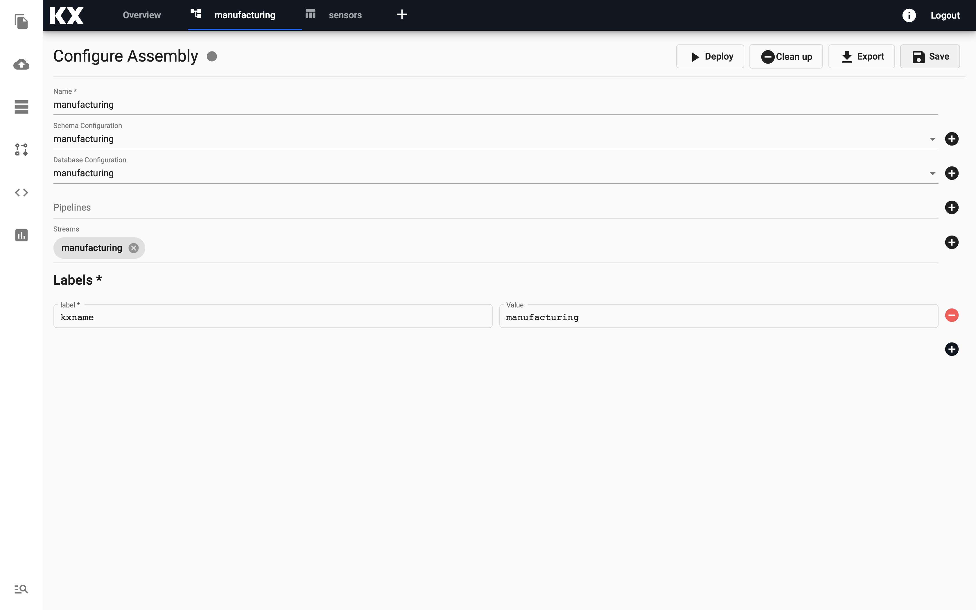
To do this, navigate back to the assembly created in the previous steps 1-4 and select the new schema in
Schema Configuration. Make sure to clickSaveto keep this change.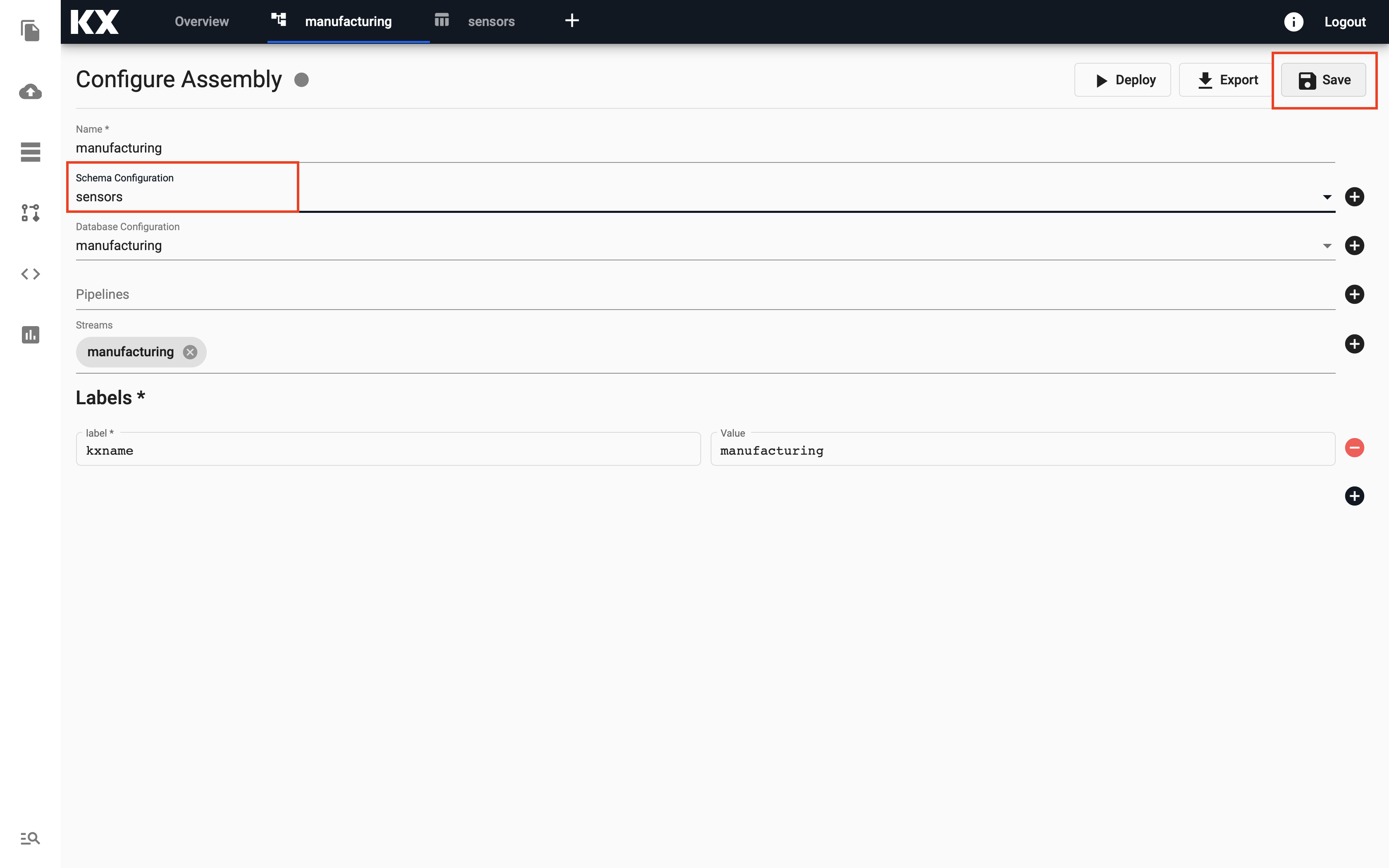
-
Select
Deploy.This takes a few seconds. When ready, the grey circle becomes a green tick and changes to
Activestatus.That's it, you are now ready to ingest data!
Step 2: Ingest live MQTT data
MQTT is a standard messaging protocol used in a wide variety of industries, such as automotive, manufacturing, telecommunications, oil and gas, etc.
It can be easily consumed by kdb Insights Enterprise. The provided MQTT feed has live sensor readings that we will consume in this recipe.
-
Select
Importfrom theGetting Startedpanel to start the process of loading in new data.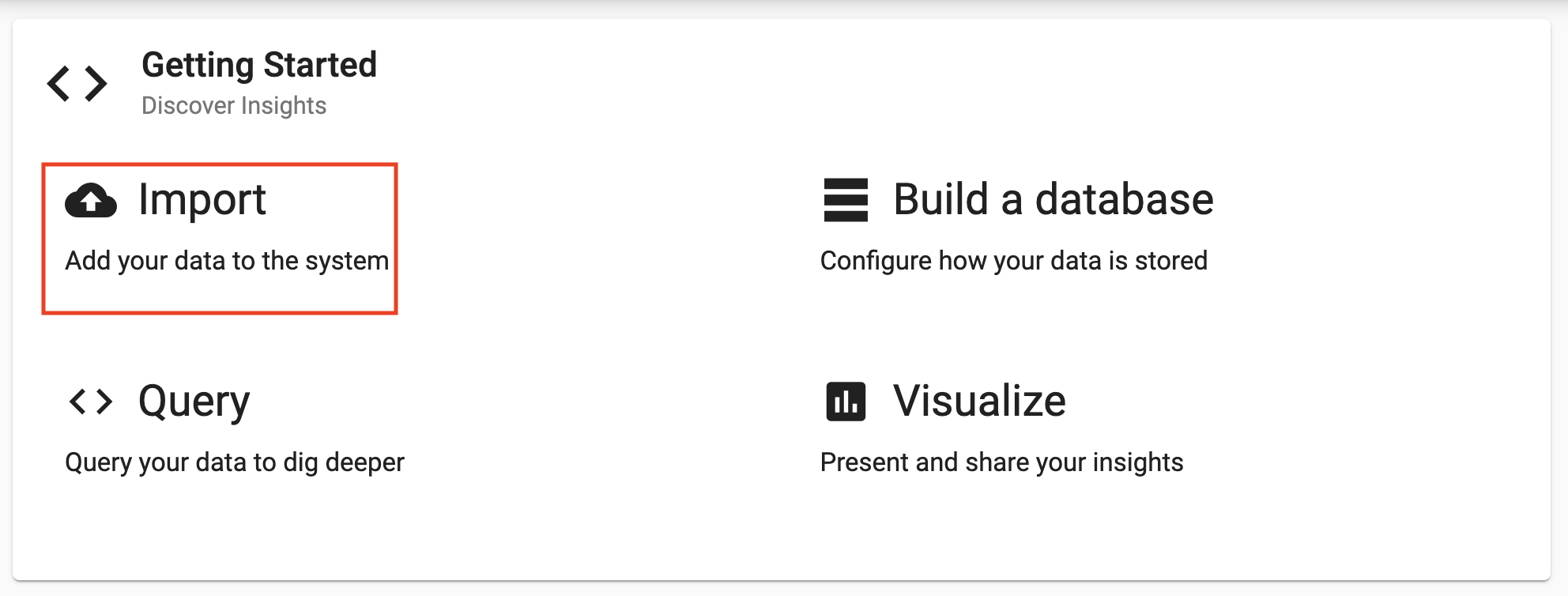
-
Select the MQTT node and enter the details as listed below to connect to the data source.
Setting Value Broker* 34.130.174.118:1883 Topic* livesensor Username* mqtt Use TLS* disabled 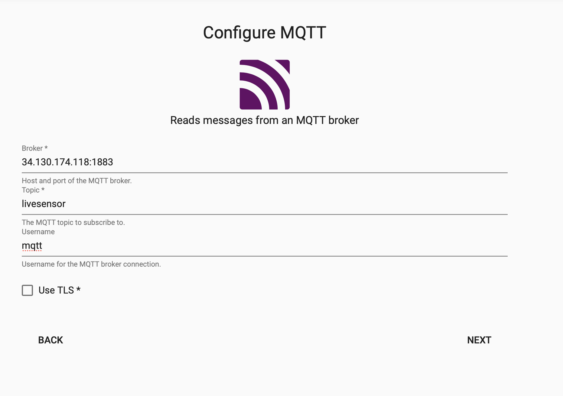
-
Select the
JSON Decoderoption and selectNext.The event data on MQTT is of JSON type so use the related decoder to transform to a kdb+ friendly format. This converts the incoming data to a kdb+ dictionary.

-
Fill in the details in the
Configure Schemascreen.This screen is a useful tool that transforms the upstream data to the correct datatype of the destination database.
- Select
Data Formatof Table from the dropdown. -
Click on the blue "+" icon next to
Parse Stringsand you will get a popup window calledLoad Schema.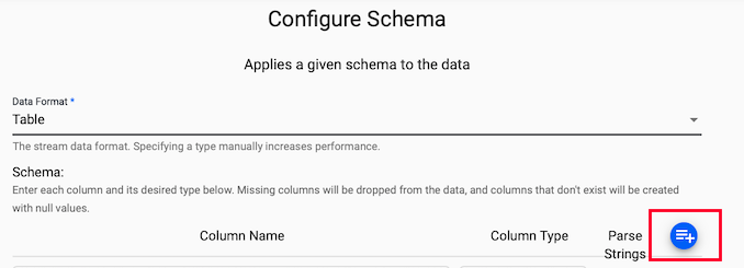
-
Select
sensorsdatabase andsensortable from the dropdown and selectLoad. -
Leave Parse Strings set to
Autofor all fields and selectNext.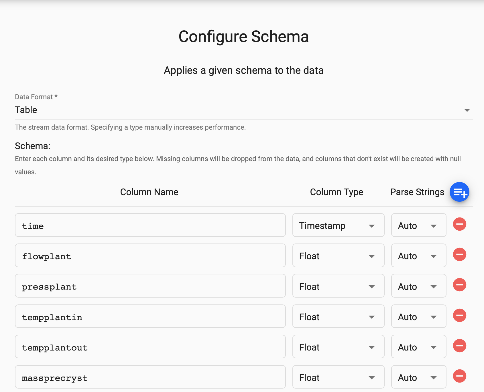
- Select
-
From the Writer dropdown select the
manufacturingdatabase and thesensorstable to write this data to and selectOpen Pipeline.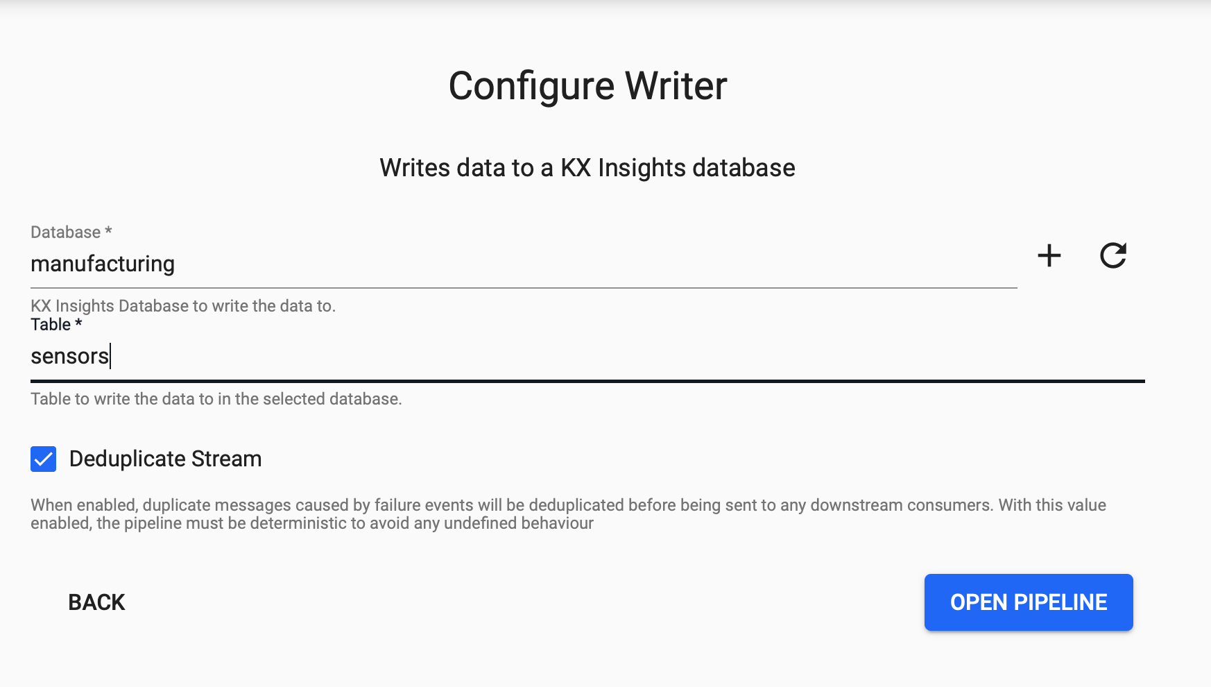
-
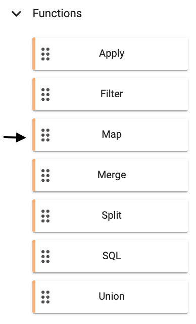
Add a new
FunctionnodeMapto the pipeline.Why do I need this?
Before you deploy the pipeline there is one more node to add. This data has been converted from incoming JSON format on the MQTT feed to a kdb+ friendly dictionary. You need to further convert this to a kdb+ table before deploying so it is ready to save to our database.
Now, transform the kdb+ dictionary format using enlist. Copy and paste the below code into your Map node and select Apply.
{[data]
    enlist data
}
You need to
Remove Edgeby hovering over the connecting line between theDecoderandTransformnodes and right clicking. You can then add in links to theFunctionmap node.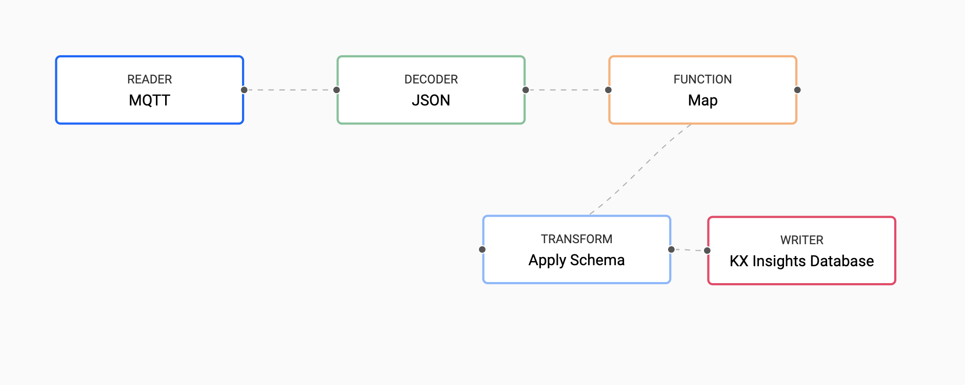
-
Click
Saveon your pipeline and give it a name that is indicative of what you are trying to do. Then you can selectDeploy.You are prompted at this stage to enter a password for the MQTT feed.
setting value password kxrecipe Once deployed you can check on the progress of your pipeline back in the
Overviewpane where you started. When it reachesStatus=Runningthen it is done and your data is loaded.Trouble deploying your pipeline?
When running
Deploy, choose theTestoption to debug each node. -
Select
Queryfrom theOverviewpanel to start the process of exploring your loaded data.-
Select Query on the top of the page. From the provided dropdowns, you can then select the table, start and end times and define a variable name that can be used in the scratchpad.
-
When you have populated the dropdowns, select
Get Datato execute the query. Data appears in the below console output.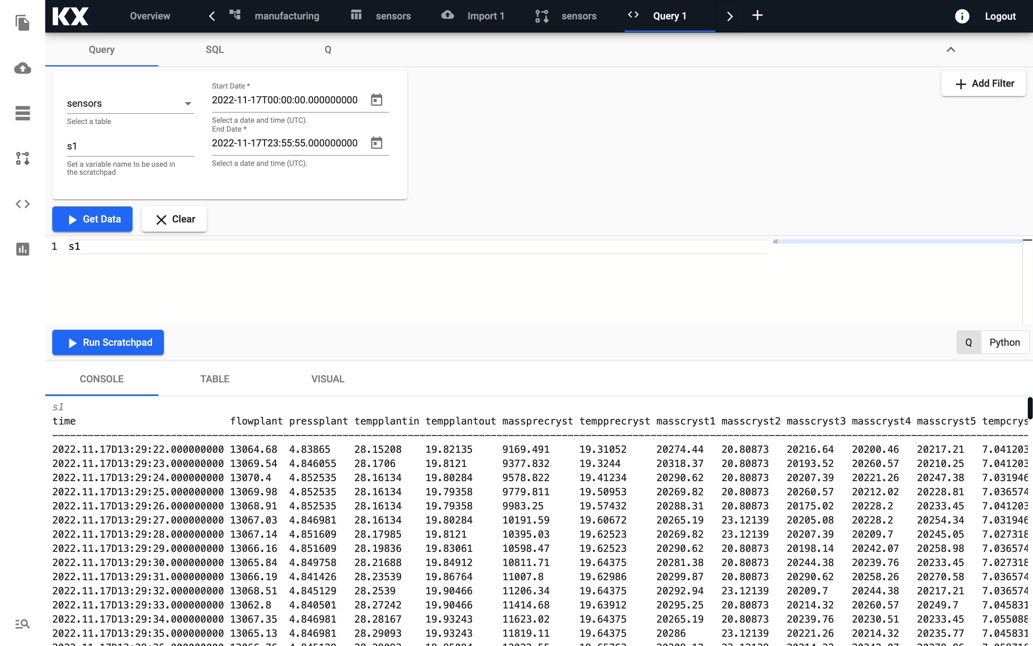
You can view the output as a Table and also as a Visual element.
-
Select the Visual tab and enter the following code to only return temperature fields.
select time,tempcryst1,tempcryst2,tempcryst3,tempcryst4,tempcryst5 from s1Select
Run Scratchpadto see the dataset plotted across time.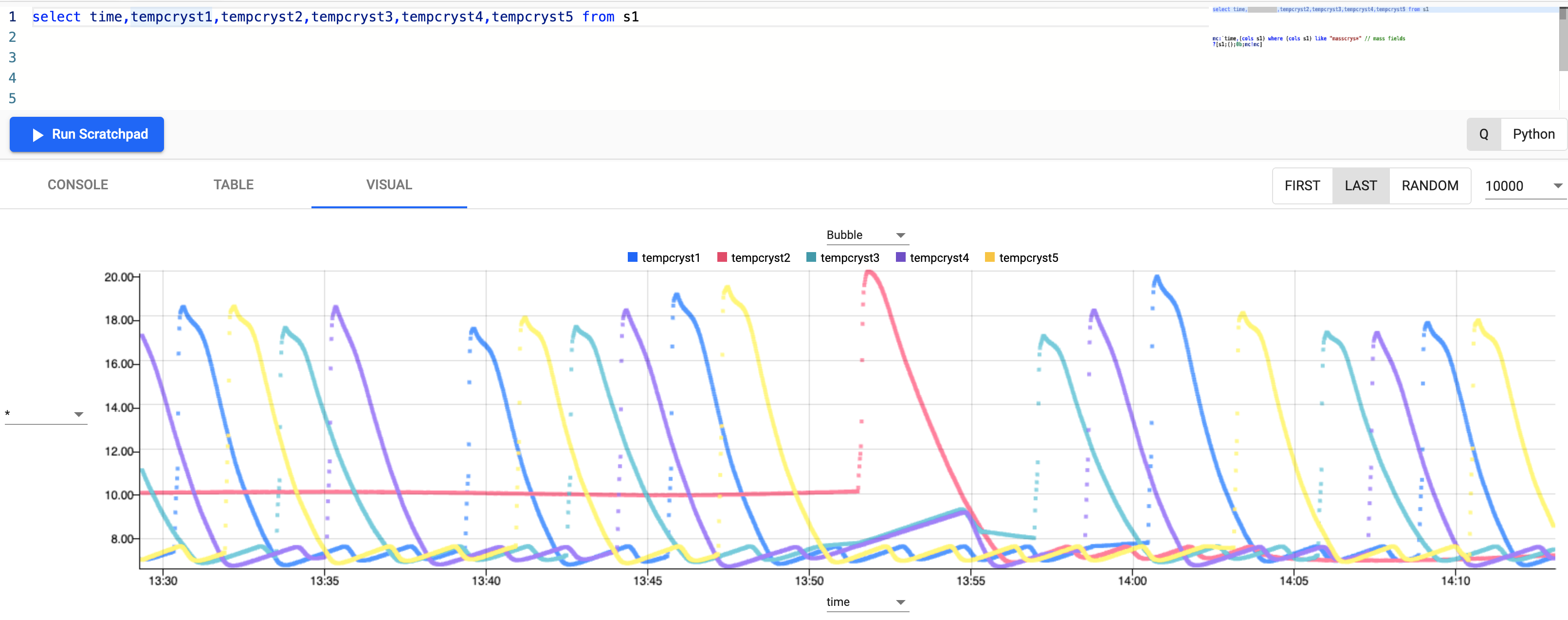
It is clear from the graph that there is a cyclical pattern to the temperature in the crystallizers fluctuating between 7-20 degrees Celcius.
-
Run a similar query but select the mass fields instead.
select time,masscryst1,masscryst2,masscryst3,masscryst4,masscryst5 from s1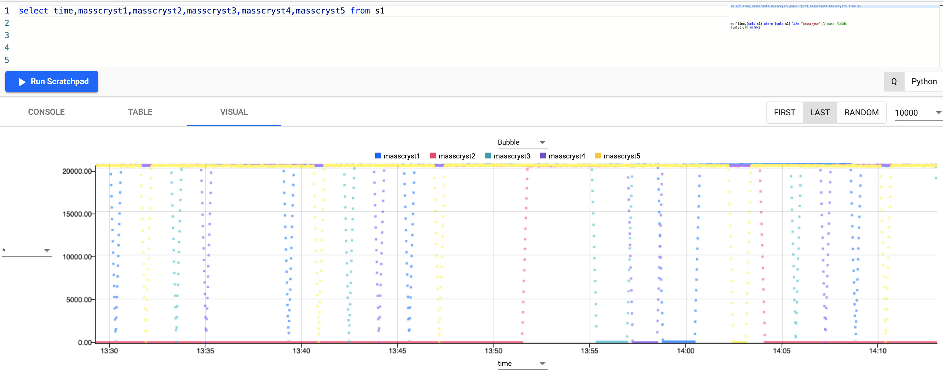
There seems to be a similar pattern to the mass levels in the crystallizers, where they are fluctuating between 0-20000kg on a cycle.
-
You have successfully setup a table consuming live sensor readings from a MQTT topic with your data updating in real time.
Step 3: Standard compute logic
-
Create control chart limit thresholds
Use Control Chart Limits to analyze data over time. It is possible to identify if process is predictable by analyzing its data, Upper Control Limit (UCL) and Lower Control Limit (LCL).
Control limits are used to avoid troubleshooting things that are not real problems on the process line. Using this chart it is possible to identify points where the process didn't match user specifications.
You will calculate the 3 sigma (three standard deviations from mean) upper and lower control limits (UCL and LCL) on one of the temperature fields. This means that 99.7% of data are within the range and outliers can be identified.
// Calculating 5 new values, most notably ucl and lcl where
// ucl - upper control limit
// lcl - lower control limit
select lastTime:last time,
    lastVal: (1.0*last tempcryst3),
    countVal: count tempcryst3,
    ucl: avg tempcryst3 + (3*dev tempcryst3),
    lcl: avg tempcryst3 - (3*dev tempcryst3)
    by xbar[10;time.minute]
    from s1
q/kdb+ functions explained
If any of the above code is new to you, don't worry, we have detailed the q functions used above:
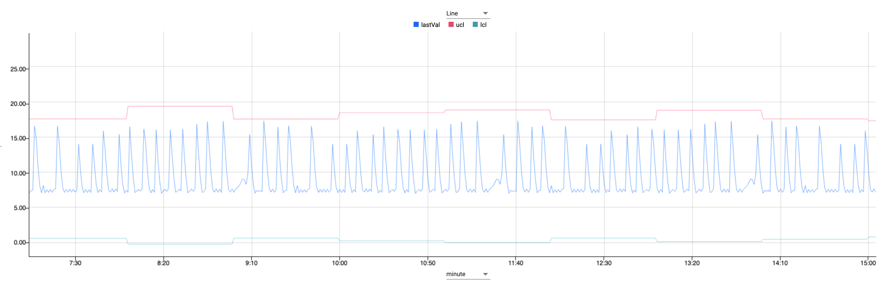
The above query selects 3 standard deviations from the average control threshold, this enables engineers to drill down into specific timeseries datapoints.
The resulting chart shows a controlled variation.

-
Aggregate over multiple time windows
Let's further extend the previous query to aggregate over two rolling time intervals. In this example we split the calculated fields with some to be aggregated over the first window (lastTime, lastVal, countVal) and the others to be aggregated over the limit fields (ucl, lcl).
// Using asof join to join 2 tables
// with differing aggregation windows
aj[`minute;
    // table 1 aggregates every 1 minute
    select lastTime : last time,
        lastVal : last tempcryst3,
        countVal : count tempcryst3
        by xbar[1;time.minute] from s1;
    // table 2 aggregates every 60 minute
    select ucl : avg[tempcryst3] + (3*dev tempcryst3),
        lcl : avg[tempcryst3] - (3*dev tempcryst3)
        by xbar[60;time.minute] from s1]
q/kdb+ functions explained
aj is a powerful timeseries join, also known as an asof join, where a time column in the first argument specifies corresponding intervals in a time column of the second argument.
This is one of two bitemporal joins available in kdb+/q.
To get an introductory lesson on bitemporal joins, view the free Academy Course on Table Joins.
This enables us to look at sensor values every minute, with limits calculated every 60 minutes providing smoother accurate more control limits.
-
Customize query by using parameters
This analytic can be easily parameterized to enable custom configuration for the end user.
// table = input data table to query over
// sd = standard deviations required
// w1 = window one for sensor readings to be aggregated by
// w2 = window two for limits to be aggregated by
controlLimit:{[table;sd;w1;w2;col1]
    aj[`minute;
    // table 1
    select lastTime : last time,
        lastVal : last tempcryst3,
        countVal : count tempcryst3
        by xbar[w1;time.minute] from table;
    // table 2
    select ucl : avg[tempcryst3] + (sd*dev tempcryst3),
        lcl : avg[tempcryst3] - (sd*dev tempcryst3)
        by xbar[w2;time.minute] from table]
}
q/kdb+ functions explained
{} known as lambda notation allows us to define functions.
It is a pair of braces (curly brackets) enclosing an optional signature (a list of up to 8 argument names) followed by a zero or more expressions separated by semicolons.
To get an introductory lesson, view the free Academy Course on Functions.
Then the user can easily change the desired windows and standard deviations required to plot variations of the dataset.
// By changing the parameter for w1 we can see the input sensor
// signal becoming smoother the larger we make it
controlLimit[s1;3;1;60]
controlLimit[s1;3;10;60]
controlLimit[s1;3;20;60]
This powerful feature enables you to calculate limits on the fly and easily customize the inputs to your own requirements.
Step 4: Apply deep neural network regression model
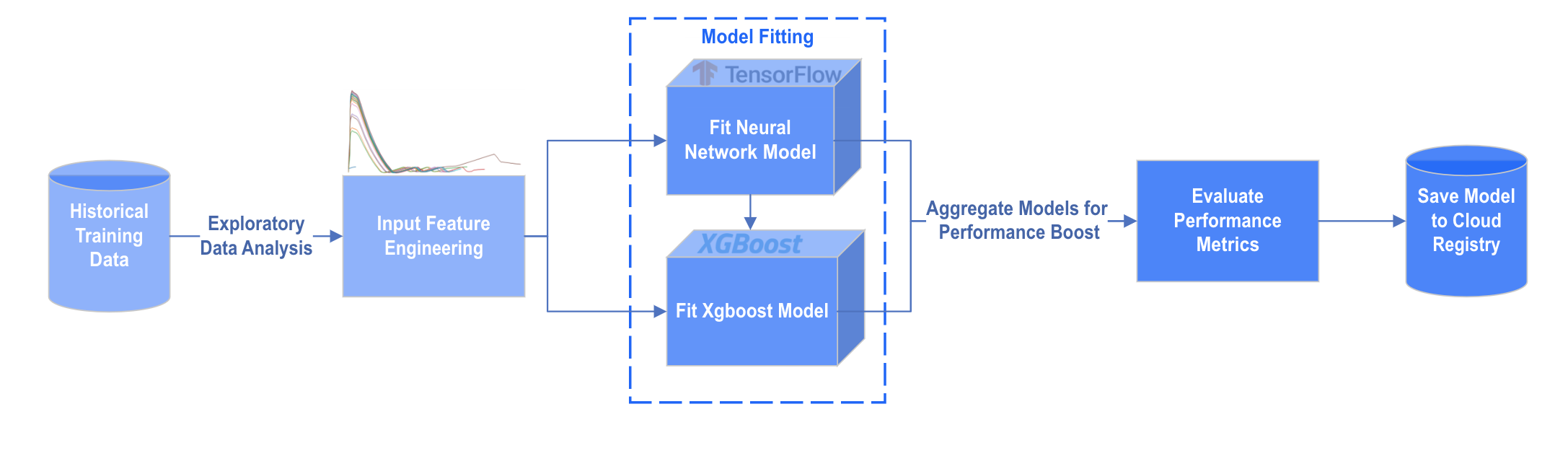
In this final stage, you will extend the pipeline created earlier in this recipe and apply a trained model stored in the cloud to the incoming streaming data.
The steps in blue in the image above are performed outside kdb Insights Enterprise. For the purposes of this recipe the model has been trained already and pushed to the Cloud Registry for you.
The model was trained used tensorflow neural networks and an xgboost model. The predictions of these two models were then aggregated to get a further performance boost.
Did you know?
It is possible to train the model inside kdb Insights Enterprise. We could even pull the training dataset directly from kdb Insights Enterprise.
We are doing this for the purposes of this recipe to make it easier for you to follow along as Machine Learning knowledge is required for the training of the model.
-
Start by duplicating the pipeline created earlier in Step 2.
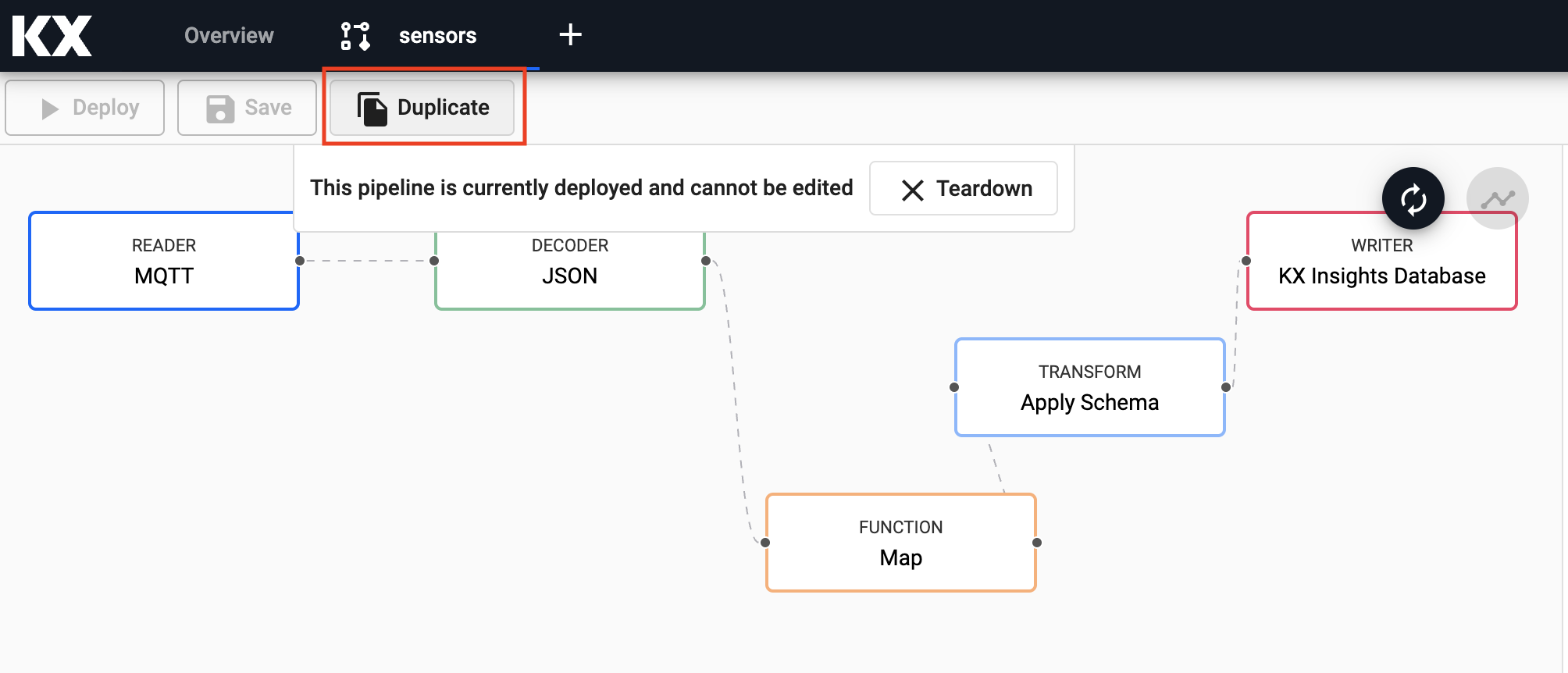
Give this a new name in the window that pops up and select
Ok. -
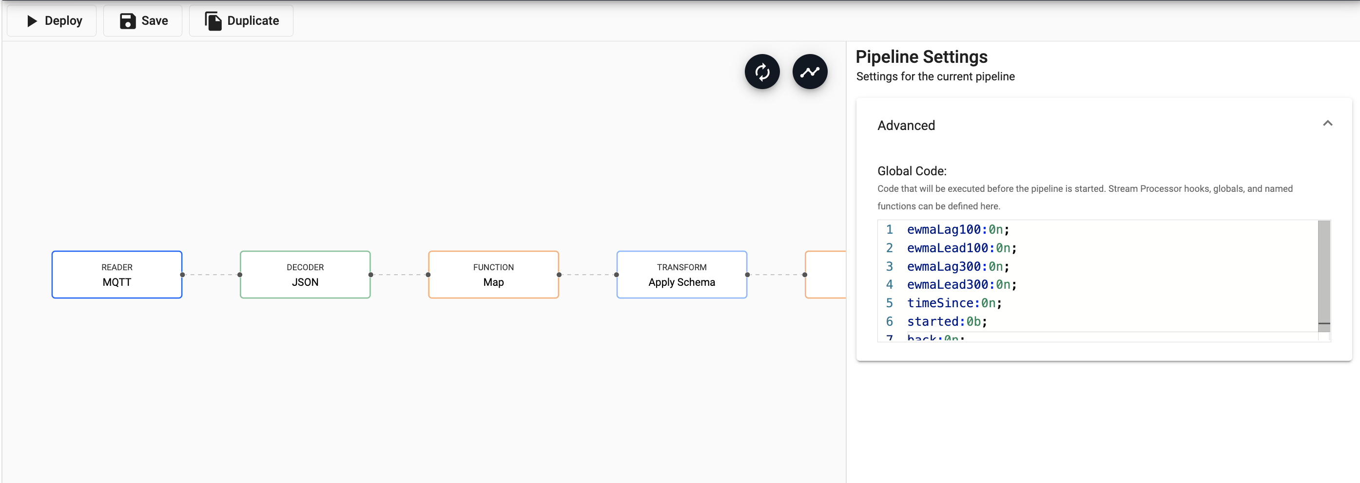
Define global variables to use in this pipeline.
To do this, click on the whitespace in the pipeline window and expand the Advanced tab.
ewmaLag100:0n;
ewmaLead100:0n;
ewmaLag300:0n;
ewmaLead300:0n;
timeSince:0n;
started:0b;
back:0n;
Copy and paste in the above code to the Global Code section in Advanced.
-
Split incoming data.
The next thing you will do is split the incoming data into two. One feeds into the KX Insights Database as before and the other makes up your new Machine Learning Workflow.
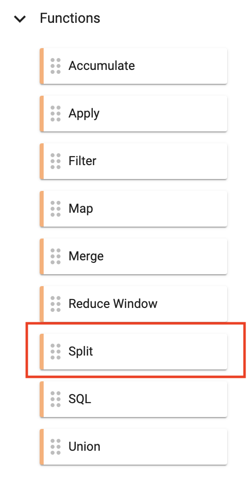
Do this by adding a Function node Split.As before you can
Remove Edgeby hovering over the connecting line between theTransformandWriternodes and right clicking. You can then add in links to theFunctionsplit node and the link back to theWriternode.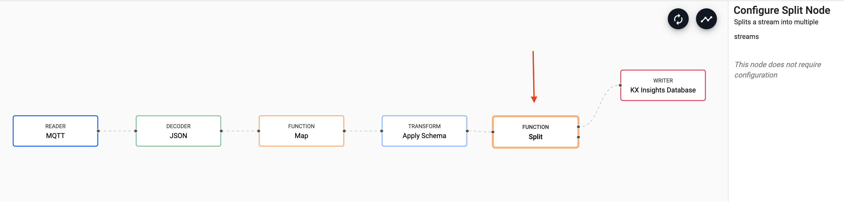
-
Add spike detection logic
Next, you will add some custom code creating new fields to calculate when the mass of the product goes from below 1000kg to above 1000kg. This is the spike threshold. It is represented in the new column
timePast, which is the time interval since the last spike.{[data] data:-1#data; $[(first[data[`masscryst3]]>1000)&(not null back)&(back<1000); [timeSince::0; back::first[data[`masscryst3]]; tmp:update timePast:timeSince from data]; [timeSince::timeSince+1; back::first[data[`masscryst3]]; tmp:update timePast:timeSince from data] ]; select time,timePast,tempcryst4,tempcryst5 from tmp }Drag in an another
Functionmap node, copy and paste in the above code and selectApply.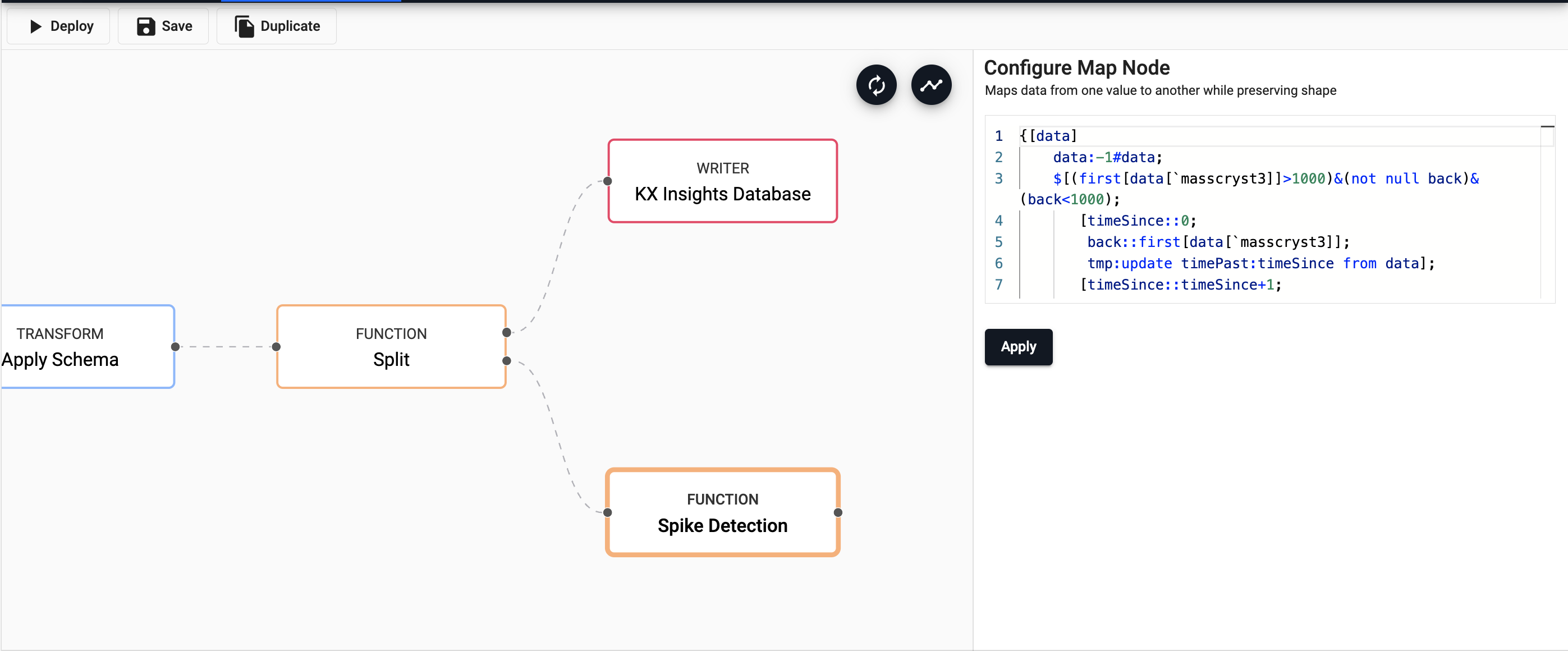
Take this opportunity to right-click the new node and rename it to something representative of its function. This is a good idea as you need to add a few more map nodes and it helps to determine which is which at a glance.
-
Add feature nodes
Next, you will add some more custom code to create some feature nodes for our model. We will calculate some moving averages of temperatures in crystallizers number 4.
{[data]
    a100:1%101.0;
    a300:1%301.0;
    $[not started;
    [ewmaLag100::first data`tempcryst5;
    ewmaLead100::first data`tempcryst4;
    ewmaLag300::first data`tempcryst5;
    ewmaLead300::first data`tempcryst4;
    started::1b];
    [ewmaLag100::(a100*first[data[`tempcryst5]])+(1-a100)*ewmaLag100;
    ewmaLead100::(a100*first[data[`tempcryst4]])+(1-a100)*ewmaLead100;
    ewmaLag300::(a300*first[data[`tempcryst5]])+(1-a300)*ewmaLag300;
    ewmaLead300::(a300*first[data[`tempcryst4]])+(1-a300)*ewmaLead300
    ]
    ];
    t:update ewmlead300:ewmaLead300,ewmlag300:ewmaLag300,ewmlead100:ewmaLead100,ewmlag100:ewmaLag100 from data;
    select from t where not null timePast
}
Drag in an another
Functionmap node, copy and paste in the above code and selectApply.
-
Pull in the machine learning model
Everything up to this point has been in preparation for this step. Now we are ready to add our Machine Learning model.
-
Drag in the
Machine Learningnode calledPredict using Registry. Click the image below to zoom in.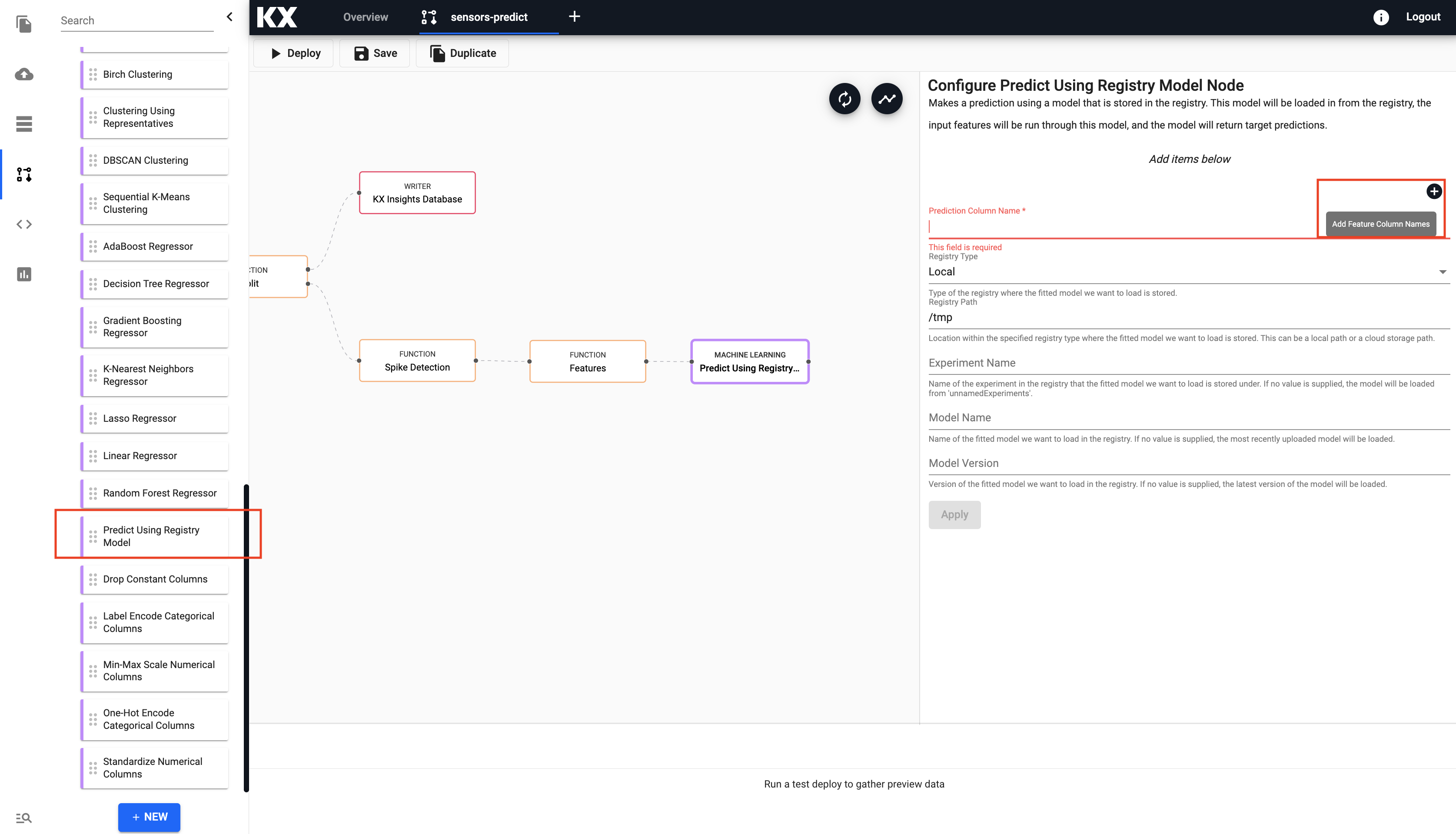
-
Select the "+" icon highlighted in the image and add the following features as calculated in the previous nodes.
-
Enter the prediction configuration details as follows and select
Apply:setting value Prediction Column Name yhat Registry Type AWS Registry Path s3://qrisk 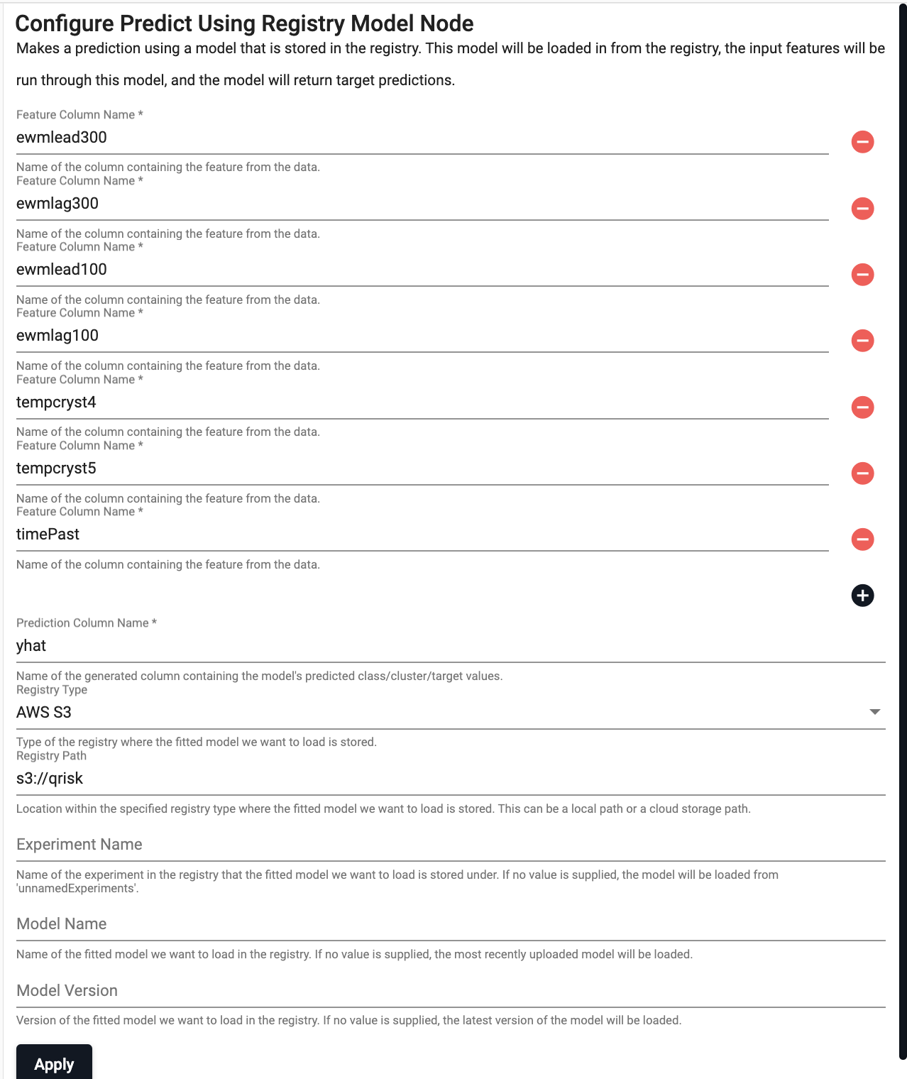
-
-
Add metadata
Next, you will add some more custom code to add some metadata.
{[data]
    tmp:?[update model:`ANN from data;();0b;`time`model`prediction!`time`model`];
    update "f"$prediction from tmp
}
Drag in an another
Functionmap node, copy and paste in the above code and selectApply.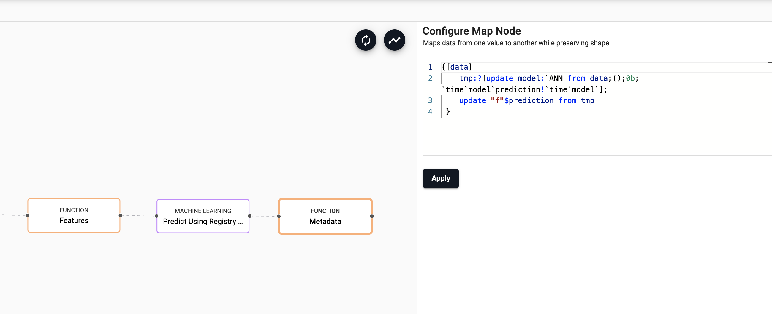
-
Write to database
Add a
Writernode to theKX Insights Database. Select themanufacturingdatabase and thepredictionstable to write this data to and selectApply.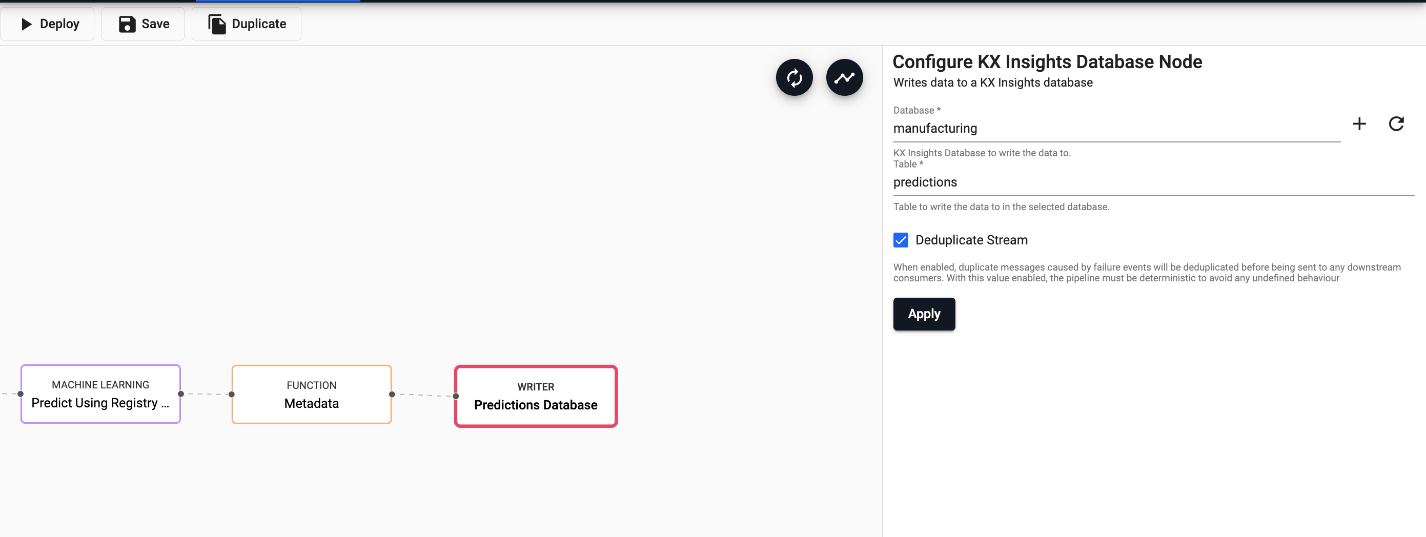
-
Define environment variables
Select
Saveand in the window that pops up select the Environment Variables option and enter the following details required to access the Machine Learning model saved on AWS Cloud Storage.variable value AWS_ACCESS_KEY_ID AKIAZPGZITYXCEC35GF2 AWS_SECRET_ACCESS_KEY X4qk/NECNmKhyO24AlEzhbzoY84bSmo7f6W7AfER AWS_REGION eu-west-1 
Select
Save. -
Deploy
If your old pipeline from Step 2 is still running, stop it by selecting
Teardownat this point before deploying the new pipeline as the steps are repeated.Now you can select
Deploy. You are prompted to enter a password for the MQTT feed.setting value password kxrecipe Once deployed, check on the progress of your pipeline back in the Overview pane where you started. When it reaches
Status=Runningthen the prediciton model has begun.When will my data be ready to Query?
It will be some time (~10-20 minutes) before the new
predictionstable is populated as the first spike in the dataset must occur before thetimePastmodel parameter is calculated. Remember, this is the time interval since the last spike.When the dataset is populated depends on the spike conditions you have set and the frequency of those occurrences in your specific dataset.
-
Query
Select
Queryfrom theGetting Startedpanel to start the process of exploring your loaded data.Select
Queryat the top of the page. From the provided dropdowns, select thepredictionstable, start and end times and define a variable name that can be used in the scratchpad.When you have populated the dropdowns, select
Visualand thenGet Datato execute the query. Data appears in the below output.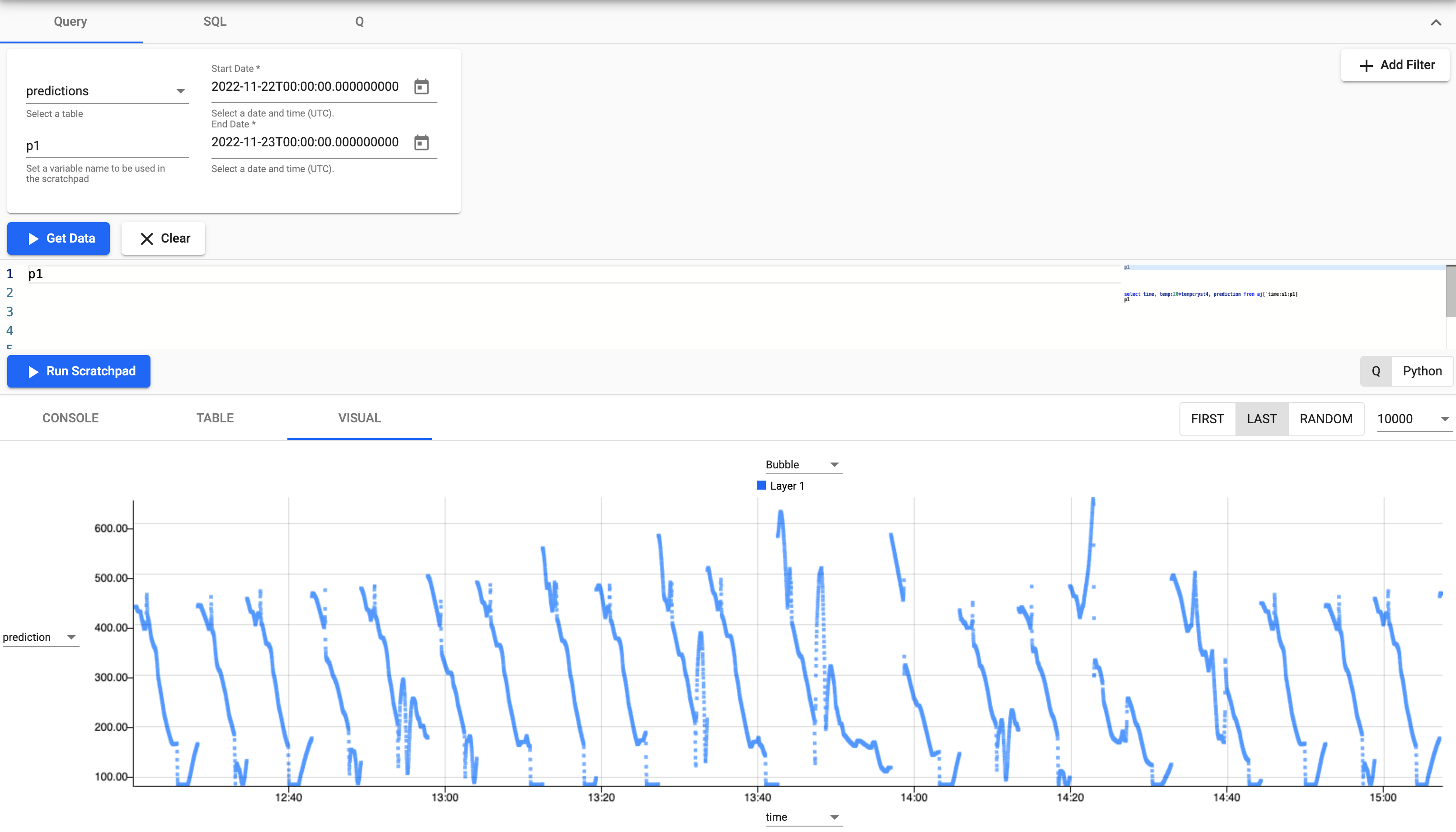
Let's next plot these predictions against the real data to see how well the model performs.
select time,
    temp:20*tempcryst4,      // adjust temp by a factor of 20 for visulization purposes
    prediction
    from aj[`time;s1;p1]        // joining sensors input data with predictions table on time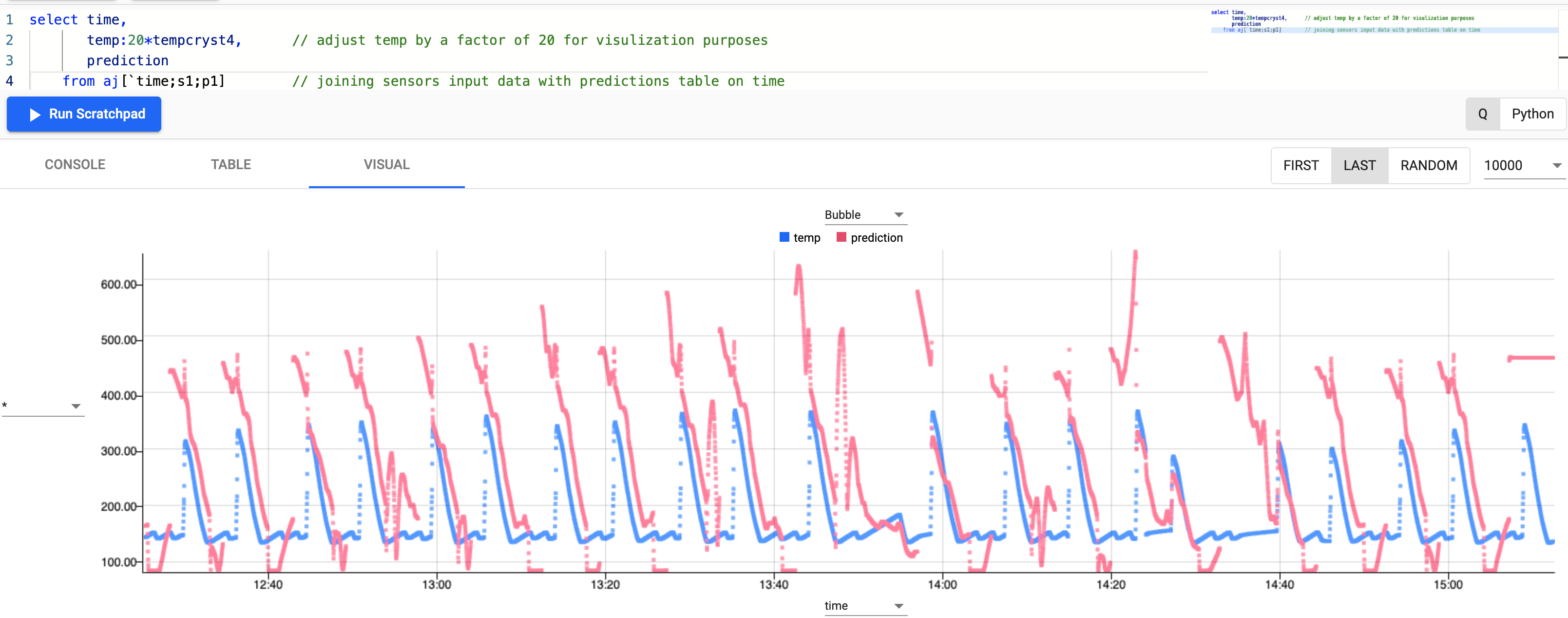
While not perfect, the model fits fairly well the incoming real dataset by how closely the red line (prediction) matches the blue line (real data). The model would perform better with more data.
This prediction gives the manufacturer advance notice of when the next cycle begins and predicted temperatures. This type of forward forecasting is useful to inform the manufacturer of the levels of filtration aids required in advance. In a typical food processing plant these levels can be adjusted in relation to the actual temperatures and pressures. By predicting these parameters before the product reaches the filters, the manufacturer can alter the dosing rate in advance and maximise throughput/yields.
This and other prediction models can save millions of dollars a year in lost profits, repair costs, and lost production time for employees. By embedding predictive analytics in applications, manufacturing managers can monitor the condition and performance of assets and predict failures before they happen.