Deliver Real-Time Insights on Streaming NYC Subway Data from Kafka
This kdb Insights Enterprise example will monitor train punctuality on the NYC subway system to better plan your travel on the network.
Find the NYC subway trains that arrive punctually and avoid those that are often delayed. See how much trains on your route are typically delayed by and plan accordingly.
Overview
Real-time data can be seamlessly handled in kdb Insights Enterprise using pipelines connecting to Apache Kafka data sources.
Connect your streaming pipelines to Apache Kafka seamlessly for maximum organizational adoption of real-time data. Apache Kafka is an event streaming platform that can be easily published to and consumed by kdb Insights Enterprise.
Benefits
| Get a Live View | Use kdb Insights Enterprise to stream data from Kafka for a continuous view of your transactional data. |
| Real Time Monitoring | View business events as they happen; be responsive not reactive. |
| Get Analytics-Ready Data | Get your data ready for analytics before it lands in the cloud. |
Subway Dataset
kdb Insights Enterprise helps users easily consume Kafka natively. We have provided a real time demo NYC subway dataset stored using Kafka; this feed offers live alerts for NYC subway trains including arrival time, stop location coordinates, direction and route details.
What questions will by answered by this Recipe?
- What was the longest stop per trip?
- Which subway train is the most punctual?
- Do the subway trains on my route typically run on time?
- What is the distribution of journeys between stations like?
Step 1: Ingesting Live Data
Deploy Database
Follow these steps to deploy the insights-demo database.
Importing Data
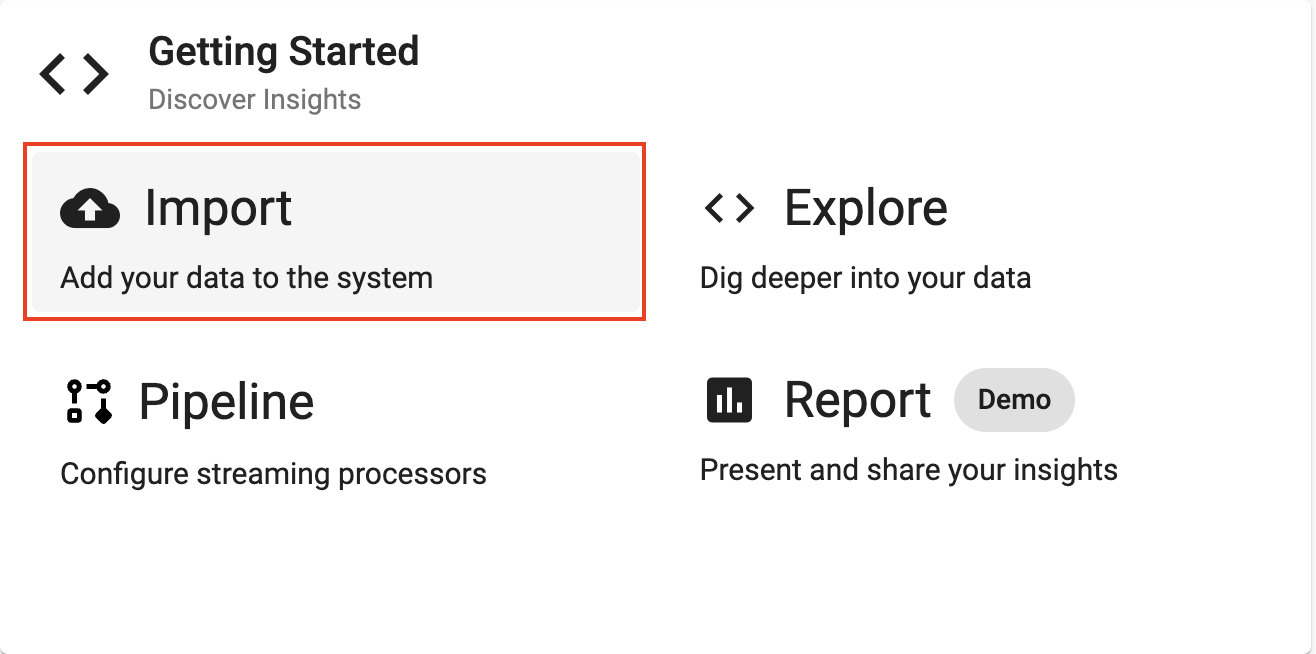
Select Import from the Overview panel to start the process of loading in new data.
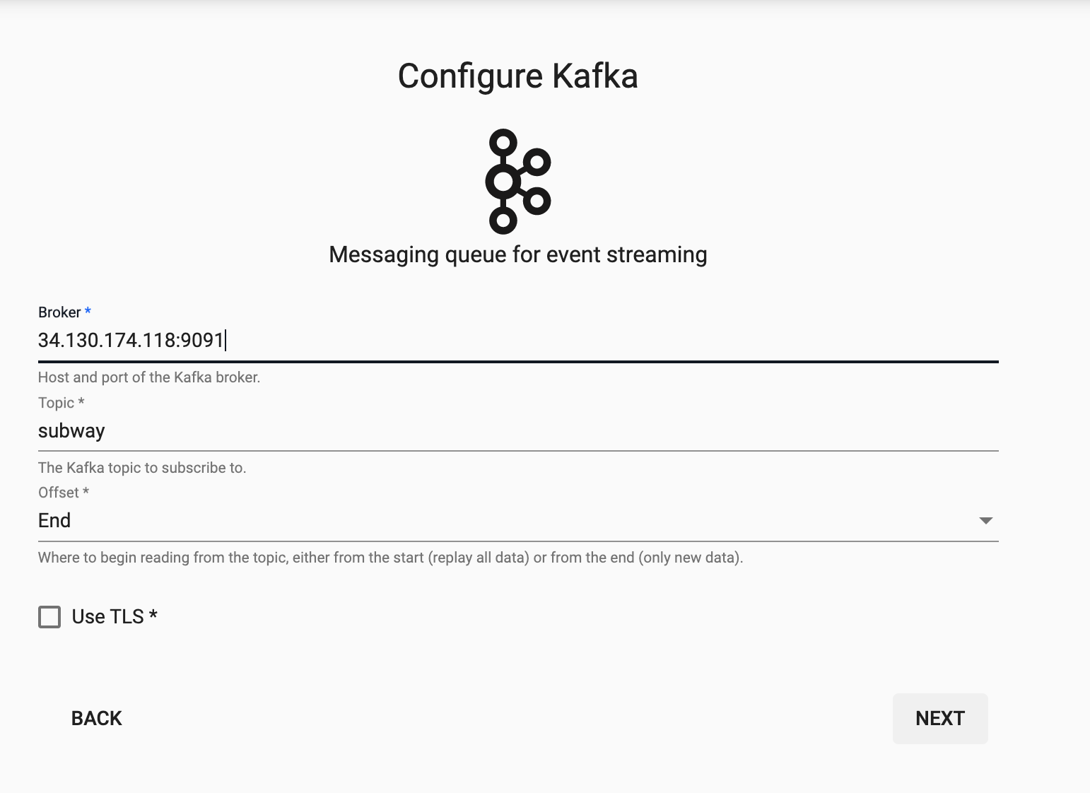
 Select the Kafka node and enter the details as listed below to connect to the datasource.
Here are the broker and topic details for the subway feed on Kafka.
| Setting | Value |
|---|---|
| Broker* | 34.130.174.118:9091 |
| Topic* | subway |
| Offset* | End |
Decoding
The event data on Kafka is of JSON type so you will need to use the related decoder to transform to a kdb+ friendly format. This will convert the incoming data to a kdb+ dictionary.
Select the JSON Decoder option.

Transforming
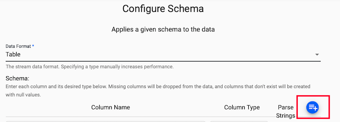
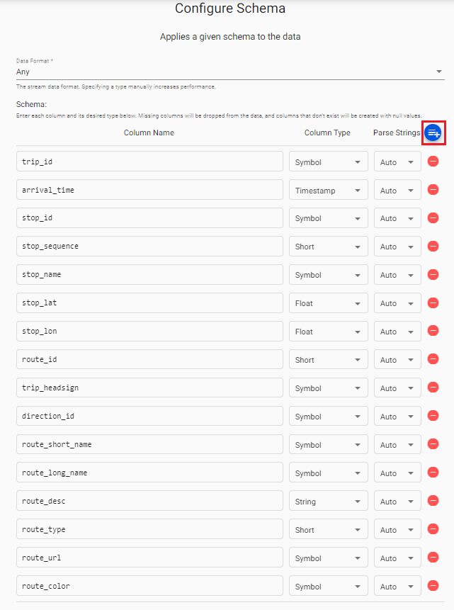
Next, we need to Configure a Schema for our data; this step transforms the upstream data to the correct kdb+ type of our destination database.
In the Apply A Schema screen select Data Format = Table from the dropdown.
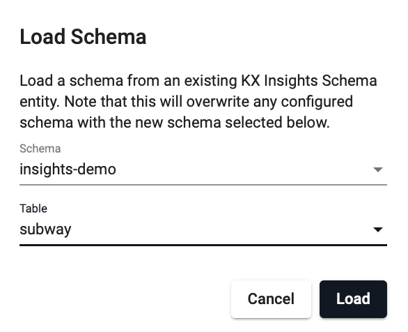
Next, click on the blue "+" icon next to Parse Strings and you should get a popup window called Load Schema.
You can then select insights-demo database and subway table from the dropdown and select Load.
Leave Parse Strings set to Auto for all fields.
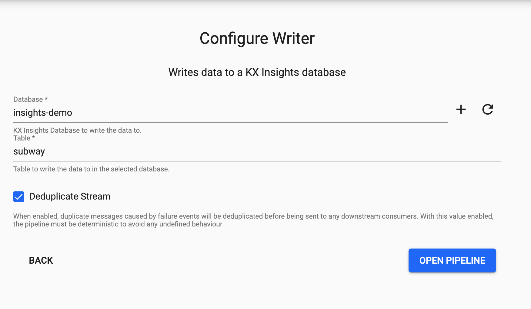
Writing
Finally, from the Writer dropdown select the insights-demo database and the subway table to write this data to and select 'Open Pipeline'.
Apply Function
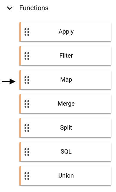
Before we deploy our pipeline there is one more node to add. This data has been converted from incoming JSON format on the Kafka feed to a kdb+ friendly dictionary.
We need to further convert this to a kdb+ table before we deploy so it is ready to save to our database. We can do this by adding a Function node Map.
Additional Functions
For readability additional nodes can be added to continue transforming the data, and moreover, if functions are predefined the name of the function can be provided here to improve reusability.
In this section you are transforming the kdb+ dictionary format using enlist. Copy and paste the below code into your Map node and select Apply.
{[data]
    enlist data
}
You will need to Remove Edge by hovering over the connecting line between the Decoder and Transform nodes and right clicking. You can then add in links to the Function map node.
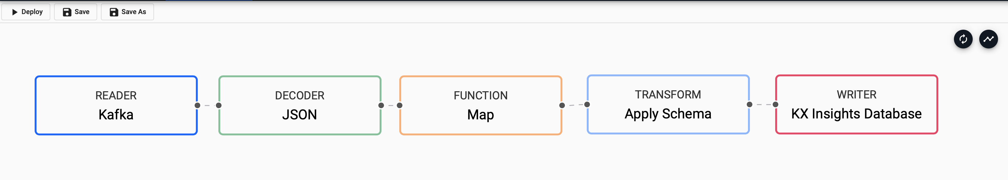
Deploying
Next you can Save your pipeline giving it a name that is indicative of what you are trying to do. Then you can select Deploy.
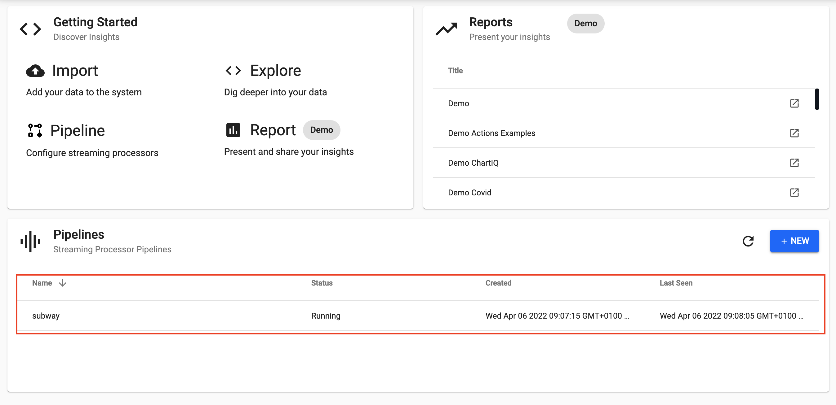
Once deployed you can check on the progress of your pipeline back in the Overview pane where you started. When it reaches Status=Running then it is done and your data is loaded.
Exploring
Select Explore from the Overview panel to start the process of exploring your loaded data.
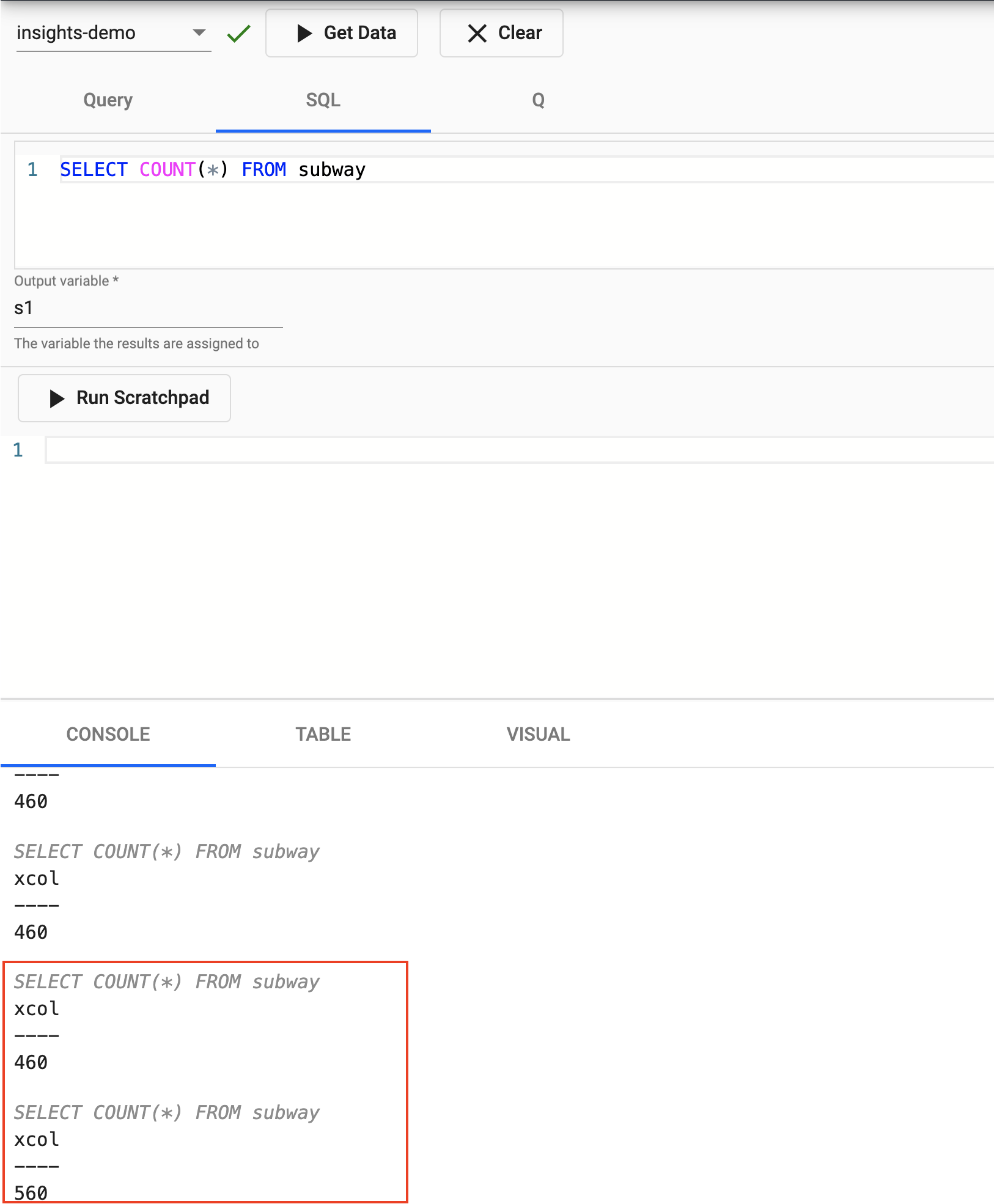
You can running the following SQL to retrieve count of the subway table.
SELECT COUNT(*) FROM subway
Rerunning this query a short while later you should notice the number increase as new messages appear on the Kafka topic and are ingested into the kdb+ table.
Nice! You have just successfully setup a table consuming live events from a Kafka topic with your data updating in real time.
Step 2: Data Analysis using Explore
Filtering & Visualising
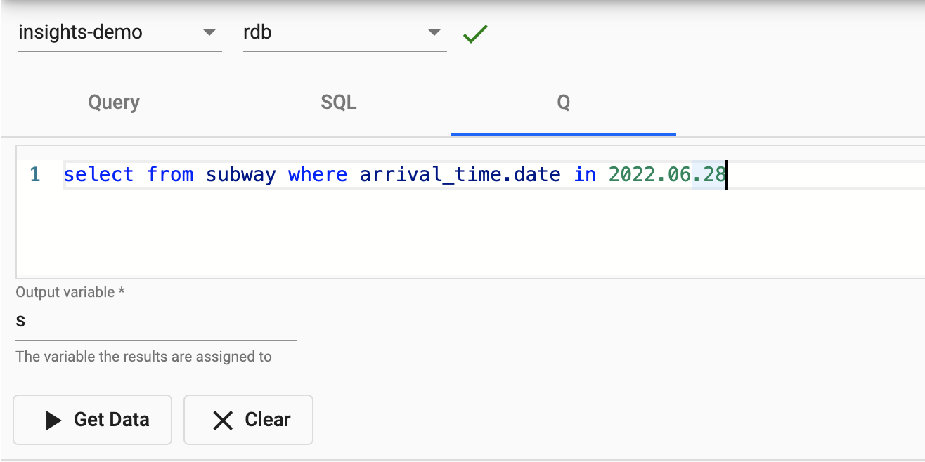
We are going to take a subset of the data for today and save that to a variable called s. Note the use of .z.d is a convienient way to return today's date.
Enter the below code into the scratchpad at the top of the page, give it a variable name s and select Get Data.
select from subway where arrival_time.date in .z.d
Now we have created the variable s which contains the subway table for todays date. We can do further analysis in memory with the scratchpad instead of directly querying the source database (more efficient and cheaper!).
Let's take a look at one only trip to start with. If the below trip_id does not exist in your table simply swap it for another.
Enter the below code into the below scratchpad and select Run Scratchpad.
select from s where trip_id like "AFA21GEN-1091-Weekday-00_033450_1..N03R"
You have the option to view the output in either the Console, Table or Visual Inspector. Note that you will have to re-run the code if you switch views.
By changing the Y axis field to be stop_sequence and the X axis field to be arrival_time we can see the subway trains journey through all its stops and how long it took.
Calculating Average Time
Let's develop this further by calculating the average time between stops per route in sequence. This metric can then be used to compare with incoming trains to determine their percentage lateness.
`arrival_time`time_between_stops xcols
    update time_between_stops:0^`second$arrival_time[i]-arrival_time[i-1] from
        select from s
            where trip_id like "AFA21GEN-1091-Weekday-00_033450_1..N03R"
New to the q language?
If any of the above code is new to you and looks a bit scary don't worry! You also have the option of coding in python.
For those that are interested in learning more, the q functions used above are:
- xcols to reorder table columns
- ^ to replace nulls with zeros
- $ to cast back to second datatype
- x[i]-x[i-1] to subract each column from the previous one
What was the longest stop for this trip?
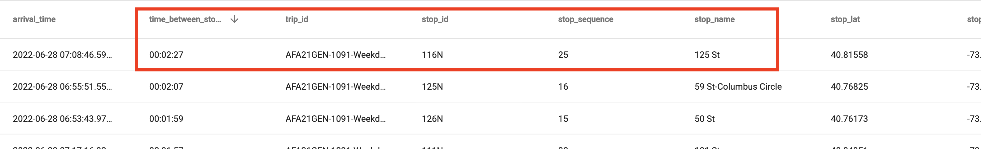
We can easily tell which stop took the longest by filtering on the newly created time_between_stops field by clicking on it in the Table tab.
We can also come to the same conclusion by switching to the Visual tab and setting the X axis as our new time_between_stops field. Note you need to rerun the query after switching views.
125 St was the longest stop
Calculating Percentage Lateness For All Trains
Next, lets look at how we can determine which trains were the best performers along their route and calculate % lateness per train.
For simplicity we will only be looking at trains that fully completed their routes.
// Getting the length of each train journey and num of stops
s3:select start_time:first arrival_time,
          journey_time:`second$last arrival_time-first arrival_time,
          first_stop:first stop_name,
          last_stop:last stop_name,
          numstops:count stop_sequence
        by route_short_name,direction_id,trip_id
        from s;
// Filtering only only trains that fully completed their route
s4:select from s3 where numstops=(max;numstops) fby route_short_name;
// Calculating the average journey time per sroute
s5:update avg_time:`second$avg journey_time by route_short_name from s4;
// Calculating the % difference between actual journey time and average time per route
s6:update avg_vs_actual_pc:100*(journey_time-avg_time)%avg_time from s5
New to the q language?
If any of the above code is new to you and looks a bit scary don't worry! You also have the option of coding in python.
For those that are interested in learning more, the q functions used above are:
- first, last to get first or last record
- - to subract one column from another
- count to return the number of records
- by to group the results of table by column/s - similar to excel pivot
- fby to filter results by a newly calculated field without needing to add it to table
- x=(max;x) to filter any records that equal the maximum value for that column
- $ to cast back to second datatype
- * to perform multiplication
- % to perform division
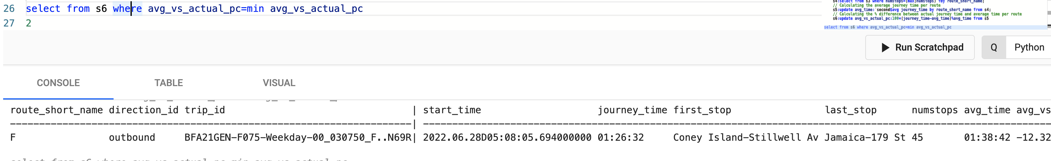
Which subway train is the most punctual?
select from s6 where avg_vs_actual_pc=min avg_vs_actual_pc
By using min we can determine that the 05:08 F train was the most punctual on this day.
Next, let's look at the result using the visual explorer for one route and try and get a sense of how trains typically run on this route.
// Filtering for at only inbound trains on Route 1
select from s6 where route_short_name=`1 ,direction_id=`inbound
Do the subway trains on my route typically run on time?
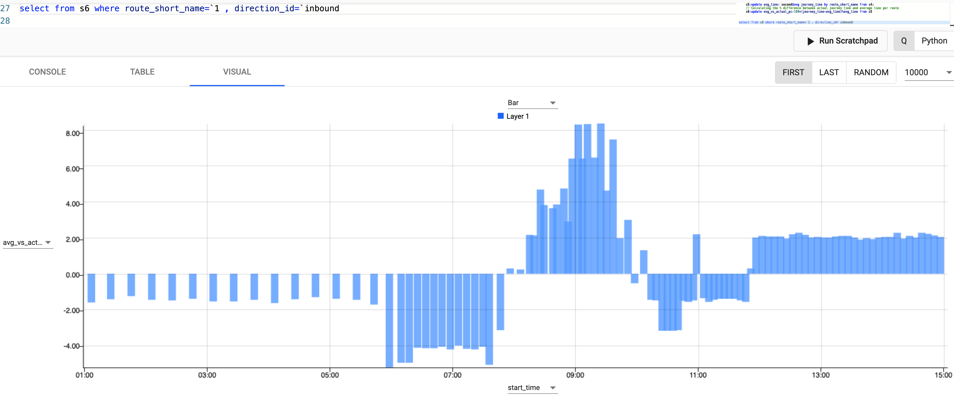 We can see from the graph above that for Route 1 typically trains before 9am are earlier on average with the worst delays between 8.20am-9.40am.
Distribution Of Times Between Stations
What is the distribution of journeys between stations like?
{count each group 1 xbar x} 1e-9*"j"$raze exec 1_deltas arrival_time by trip_id from s
We can see from the histogram chart that journeys between stations run along scheduled time intervals of 60, 90 and 120 seconds, with the most common journey time between stations of approximately 60 seconds.
