An introduction to neural networks with kdb+
Due to the desire to understand the brain and mimic the way it works by creating machines that learn, neural networks have been studied with great interest for many decades. A simple mathematical model for the neuron was first presented to the world by Warren McCulloch and Walter Pitts in 1943.
With modern advances in technology and the computational power available, this field of research has had massive implications on how computers can be used to ‘think’ and learn to solve problems given an appropriate algorithm. A few interesting examples of this research in action include:
-
Interpreting art and painting images [Mordvintsev et al.] [Gatys et al.]
A number of different algorithms have been developed around this field of research, and this paper is going to focus on the implementation of a feedforward neural network in kdb+. A feedforward network (also known as a multi-layer perceptron) is a type of supervised machine-learning algorithm which uses a series of nonlinear functions layered together with an output. It can be used for classification or regression purposes and has been shown to be a universal approximator – an algorithm that can model any smooth function given enough hidden units.
Reference
See Kurt Hornik, “Approximation Capabilities of Multilayer Feedforward Networks”, Neural Networks, Vol. 4, pp. 251-257, 1991
This design of feedforward networks can be represented through operations on matrices and vectors. Array-programming languages such as q are well suited to computational implementations in this format due to the vectorized operations on lists.
All tests were run using kdb+ version 3.2 (2015.05.07)
Feedforward networks
As mentioned in the introduction, a feedforward neural network is a type of supervised machine-learning algorithm. This means that it is trained on datasets for which the output for given inputs is already known.
A neural network consists of a set of neurons connected together in some order. Each neuron receives inputs from other neurons, performs some action on these inputs and outputs a signal that becomes input for another connected neuron.
The perceptron
A single neuron by itself is often referred to as a perceptron (Figure 1). The idea is to construct a predictor based on a linear combination of the inputs and a set of weights which control the impact an input has on the system. This linear combination (the dot product of the inputs and the weights) is then used as the input to a chosen threshold function which produces the desired output.
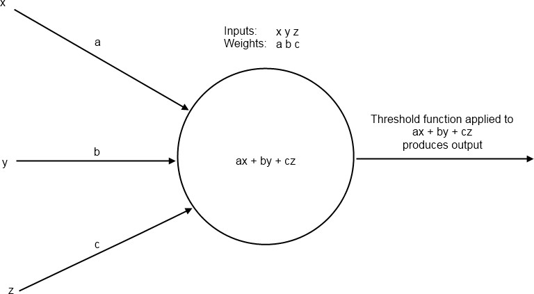
Figure 1: A perceptron
Threshold function
A threshold function represents the activation of the perceptron based on its inputs. A common choice for this function is the sigmoid function.
q)sigmoid:{1%1+exp neg x}
q)output:sigmoid[inputs mmu weights]
This function provides a smooth curve bounded asymptotically by 0 and 1 on the vertical axis (Figure 2).
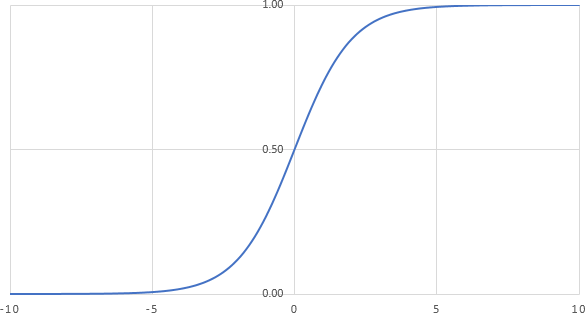
Figure 2: A plot of the sigmoid function
Perceptrons as linear predictors
Perceptrons can only solve linearly-separable problems. A linearly-separable problem is one where two sets in a plane can be cleanly divided by a straight line. We can demonstrate this by looking at plots of truth table outputs.
Let us say that a red dot represents true and a blue dot represents false. If we take the standard truth table inputs of 1 or 0 and add some random noise to them so that they are either slightly smaller than 1 or slightly larger than 0, then we get the plots shown in Figure 3.
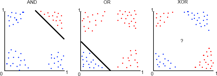
Figure 3: Truth Table Plots
Notice how we can easily separate the true results from false in the AND and OR truth tables with a straight line. Perceptrons are good predictors for these problems. However, if the data is not so easily separable, as with the XOR plot, we need a way to be able to make nonlinear predictions. Solving the XOR problem will form our motivation for connecting many perceptrons into a network.
A neural network
A network consists of neurons connected together in layers as shown in Figure 4. Each neuron in one layer is connected to each neuron in the next layer and each connection has an associated weight. The first layer of neurons is the input layer. The neurons in this layer represent input values from a data sample.
Following the input layer are the hidden layers. The number of neurons in a hidden layer is determined through a combination of background understanding of the problem and trial and error.
Finally there is the output layer. The number of neurons in this layer is determined by the type of problem to be solved. For example one might wish to classify an input data sample into one of two categories (e.g. true or false as in the XOR problem). This type of problem is referred to as a binary classification problem. For this type of problem we only need one output neuron because the sigmoid function will return values close to 1 or 0 after the network is trained.
However, the function which acts on the linear combination of inputs and weights at the output layer is not always the same as the threshold function used throughout the rest of the network. This is because we do not always desire a value between 0 and 1. Output functions for addressing different types of problems will be discussed in detail in Output functions for regression and multi-class classification.
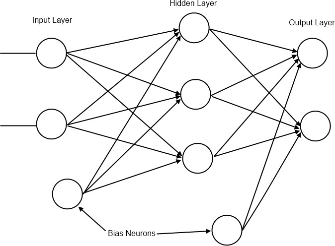
Figure 4: A feedforward network
Bias neurons
A bias neuron is a neuron external to the main network. One is added to the input layer and one to each of the hidden layers. The value it passes to neurons in the next layer is always 1 and it receives no inputs from previous layers (see Figure 4). The purpose of bias neurons is analogous to the intercept parameter of a simple linear model – commonly written as
The absence of \(\beta_{0}x_{0}\) in the simple linear model results in the predicted line always passing through (0, 0) and the model will perform poorly when attempting to predict unknown values. Hence we always set \(x_{0}\) to 1 and alter \(\beta_{0}\) as we find the line of best fit. In the neural network we represent the network’s version of the \(\beta_{0}x_{0}\) term as a bias neuron and associated weights. For more information on bias terms in statistical modelling see Chapter 3 in [2] and Chapter 7 in [1].
Bias neurons are added to the input layer by adding a 1 to each of the input samples in the data set used to train the network.
// Inputs and expected target values for XOR problem
q)input:((0 0f);(0 1f);(1 0f);(1 1f))
// Add a bias neuron to each input
q)input:input,’1.0
q)target:0 1 1 0f
Weight initialization
The initialization process begins by assigning values to the weights present in the network. The weights are randomly assigned such that the values of the weights between the input nodes and a receiving node on the next layer are in the range (-1, 1) with mean 0.
Since there will be multiple neurons in the next layer we can represent all the weights between two layers as a matrix, where the number of rows represents the number of inputs and the number of columns represents the number of neurons in the next layer. An example of how this weight matrix and the input matrix interact is shown in Figure 5.
wInit:{
  // If only one input neuron is detected exit
  // This is most likely due to a missing bias neuron
  if[1=x;:"Number of input neurons must be greater than 1."];
  flip flip[r]-avg r:{[x;y]x?1.0}[y]each til x
  }
Initialize weights between three inputs and four outputs. The first column represents the weights (connections) between the three inputs and the first neuron in the next layer. The second column is the weights leading to the second neuron in the next layer and so on.
q)wInit[3;4]
-0.3586151 0.09051553 -0.2815408 -0.05282783
0.02154042 0.4219367  0.2320934  -0.05853578
0.3370747  -0.5124522 0.04944742 0.1113636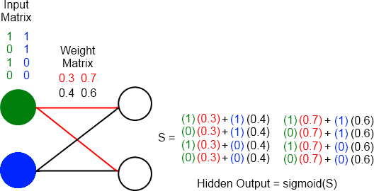
Figure 5: Diagram showing 2 input neurons (green and blue neurons)
connecting to 2 hidden neurons. The colors in the matrices correspond
to the area of the network those values are found during execution
of a forward pass.
The feedforward network in kdb+
Once we have prepared the input data and the weights they can be applied to the network to provide output. We will use the network to predict the outputs of the XOR function.
// weights between input layer and hidden layer (2 inputs + 1 bias neuron)
 q)w:wInit[3;4]
// weights between hidden layer and output layer (4 hidden neurons + 1 bias neuron)
 q)v:wInit[5;1]
 q)ffn:{[input;w;v]
// Apply inputs and their weights to the hidden layer
   z:sigmoid[input mmu w];
// Use output from hidden layer to generate an output
   sigmoid[z mmu v]
  }
 q)ffn[input;w;v]
 0.5028818
 0.5136649
 0.4891303
0.5
The network has produced an output, but these values are not close to the target values. This is understandable as the weights have been randomly initialized. In order to produce the desired output the network must learn a more appropriate set of weights.
Training the network
Training a network to produce accurate results involves determining the weights which minimize the errors of the output nodes. The problem of minimizing the error by adjusting the weights is solved by a technique called back-propagation – a form of gradient descent.
Gradient descent begins by calculating the derivative of the error function with respect to the weights. This derivative gives information about the direction needed to move along the surface described by the error function in order to arrive at a minimum. The weights are gradually adjusted using this information until an acceptable minimum in error has been reached.
Back-propagation
Back-propagation trains the network by propagating information about the error at the output back through the network and adjusting all the weights of the connecting neurons. For an output node that applies the sigmoid function the error function is the cross-entropy error function defined as:
This gives us the following update rule for adjusting the weights between the output node and the hidden layer:
where:
- \(z^{t}_h\)
-
the output after evaluating the hidden neuron \(h\) for input sample \(t\)
- \(v_h\)
-
the weight between the output neuron and hidden neuron \(h\)
- \(y_t\)
-
the target for sample \(t\)
- \(\widehat{y}^t\)
-
the calculated output for sample \(t\)
- \(\alpha\)
-
the rate at which we adjust the weights (usually < 0.1)
Update rules
The derivation of the update rules for back-propagation is beyond the scope of this paper. See Chapter 11 in [3] and Chapter 11 in [2].
Once the change in the above weights has been calculated we propagate the error to the hidden layer and generate the update rule for the weights between the input layer and the hidden layer:
where:
- \(w_{hj}\)
-
the weight between hidden neuron \(h\) and input neuron \(j\)
- \(x^t_j\)
-
the input from neuron \(j\) for some sample \(t\)
Using these formulas we can update our feedforward network function to implement back-propagation and allow training:
// inputs - the input data set with bias node
// targets – known outputs corresponding to inputs
// lr – learning rate ‘alpha’
// d – dictionary with 3 items: output
//     weights between input and hidden layers
//     weights between hidden and output layers
ffn:{[inputs;targets;lr;d]
  z:1.0,/:sigmoid[inputs mmu d`w];
  o:sigmoid[z mmu d`v];
  // Error of output neurons
  deltaO:(targets-o);
  // Error of hidden neurons
  deltaZ:1_/:$[deltaO;flip d`v]*z*1-z;
  `o`v`w!(o;d[`v]+lr*flip[z]      mmu deltaO;
            d[`w]+lr*flip[inputs] mmu deltaZ)
  }
// Example – the XOR problem
q)inputs
0 0 1
0 1 1
1 0 1
1 1 1
q)targets
0 1 1 0f
q)w
0.3257579 0.348099 -0.4320058 0.3356597
-0.07237444 -0.3028193 0.3088185 -0.3069554
-0.2533834 -0.04527963 0.1231874 -0.02870423
q)v
-0.0133154
0.04739764
0.2894549
-0.3235371
// Two training passes show little change
q)finalResult:(ffn[inputs;targets;0.1]/)[2;`o`w`v!(0,();w;v)]
q)finalResult`o
0.5025557
0.5133001
0.4888265
0.4996545
// 10000 training passes shows significant improvement
q)finalResult:(ffn[inputs;targets;0.1]/)[10000;`o`w`v!(0,();w;v)]
q)finalResult`o
0.009305227
0.9890354
0.9890087
0.01142469
q)\ts finalResult:(ffn[inputs;targets;0.1]/)[10000;`o`w`v!(0,();w;v)]
164 2992// generate a random permutation of list 0 to 99
q)rp:-100?til 100
// use rp to shuffle inputs and targets
// we generate rp first so that the shuffled indices of
// the inputs and targets match up
q)inputs:(100#inputs)rp
q)targets:(100#targets)rp
// using weights of trained network solve test inputs
q)rw:finalResult`w; rv:finalResult`v
q)res: (ffn[inputs;targets;0.1]/)[1;`o`w`v!(0;rw;rv)]
// Are all the predictions correct?
q)all raze[`int$res`o]=targets
1bOutput functions for regression and multi-class classification
There are three types of output we are looking for when using a network of this type. The first we have already discussed in A neural network above – binary classification. We have also worked through an example of this problem when applying the network to predict XOR outputs. The other two problems we will discuss are multiclass outputs and nonlinear regression outputs.
Multiclass outputs
For multiclass outputs the goal is to determine the correct classification of an input into three or more possible classifications. Unlike the binary classification situation, in the output layer there will be one neuron for each possible classification. The target values are transformed using one-hot encoding. This gives us a unique list of 0s and 1s for each possible classification that is the same length as the number of possible classifications. For example, if there are classifications A, B and C the transformations are 0 0 1, 0 1 0 and 1 0 0 – giving the output layer target patterns to match for training and testing. The output function used is the softmax function:
where
- \(\widehat{y}^t_i\)
-
the output from neuron \(i\) for sample \(t\)
- \(S^t_i\)
-
the linear combination of outputs from the hidden layer and the weights connecting the hidden layer to output neuron \(i\) for sample \(t\)
- \(S^t_k\)
-
the linear combination of outputs from the hidden layer and the weights connecting the hidden layer to output neuron \(k\) for sample \(t\)
By using the softmax function we ensure that the sum of the outputs from each of the neurons in the output layer is 1. That allows us to pick the neuron with the highest output value as the most likely to be the classification we expect for the given input; the ‘winning’ neuron will be assigned a value of 1 and the other neurons a value of 0 resulting in a match to one of the one-hot encoded classifications. The cross-entropy error function in this case is:
where \(\widehat{y}^t_i\) is the target value for output neuron \(i\) with sample \(t\).
The update rules are:
where \(v_{ih}\) is the weight between output neuron \(i\) and hidden neuron \(h\).
An example implementation of the softmax output is shown below in Classification for 3+ classes.
Nonlinear regression outputs
If the goal is to predict a real value, not necessarily constrained within the boundaries imposed by a threshold function, the output function is just the linear combination of the outputs from the hidden layer.
where
- \(\textbf{v}\)
-
the vector of weights between the hidden layer and the output layer
- \(\textbf{z}^t\)
-
the vector of outputs from the hidden layer
In this case we change the error function from cross-entropy to the sum-of-squared errors:
The update rules for a regression output are:
q)lin:{x}
q)linErr:{0.5*sum sum a*a:x-y}
It’s useful now to put the different functions for error and output in
dictionary format as this will allow us to use the same ffn function
for all 3 types of classification:
// x is linear combination of hidden outputs and weights
outputFuncs:`sig`smax`lin!
  ({1%1+exp neg x};{exp[x]%sum flip exp x};{x})
// x is target value, y is calculated
errFuncs:`sig`smax`lin!
  ({neg sum sum flip(x*log y)+(1-x)*log 1-y};
  {neg sum sum flip x*log y};
  {sum sum a*a:x-y})
ffn:{[inputs;targets;lr;of;d]
// Calculate the outputs of the hidden layer
// and add bias node
z:1.0,/:sigmoid[inputs mmu d`w];
o:outputFuncs[of][z mmu d`v];
// Error of output neurons
deltaO:(targets-o);
// Error of hidden neurons
// Hidden bias node is not connected to any
// input layer nodes so we drop it
deltaZ:1_/:$[deltaO;flip d`v]*z*1-z;
`o`v`w`err!
(o;
d[`v]+lr*flip[z] mmu deltaO;
d[`w]+lr*flip[inputs] mmu deltaZ;
errFuncs[of][targets;o])
}Classification for 3+ classes
As an example, we will study a set of Iris flower data which was originally introduced into research by Ronald Fisher in 1936. It contains samples from three different species of the Iris flower and has become a standard test case for many classification techniques within machine learning. By taking measurements of certain metrics (eg. length and width of sepals) the plants can be classified and computationally distinguished from each other. The data and a description of the data can be found in the links at archive.ics.uci.edu
We one-hot encode the different possible species of Iris, resulting in a neural network with 5 inputs (including the bias neuron), 7 hidden neurons (including the bias neuron) and 3 outputs. The data set is randomly shuffled to reduce the likelihood of a biased output. From this randomized selection of the data a random selection of 20 samples is taken as the test set and the other 130 samples are used in training.
// one-hot encoding of classes
q)IrisOneH:oneHot[distinct Iris.species]
q)IrisOneH
Iris-setosa    | 1 0 0
Iris-versicolor| 0 1 0
Iris-virginica | 0 0 1
q)Iris1h
slength swidth plength pwidth species     onehot
------------------------------------------------
5.1     3.5    1.4     0.2    Iris-setosa 1 0 0
4.9     3      1.4     0.2    Iris-setosa 1 0 0
4.7     3.2    1.3     0.2    Iris-setosa 1 0 0
..
// Random permutation of the dataset
q)IrisRP:Iris1h{neg[x]?til x}count Iris1h
// Pick a test set – samples from data not used in training
q)IrisTest:IrisRP[-20?count IrisRP]
q)IrisTrain:IrisRP except IrisTest
// Init weights, input and output variables
q)w:wInit[5;6]
q)v:wInit[7;3]
q)input:1.0,'flip flip[IrisTrain]`slength`swidth`plength`pwidth
q)output:IrisTrain.onehot
// Train network
q)resIris:(ffn[input;output;0.01;`smax]/)[800;`o`w`v`err!(0;w;v;1f)]
// After 800 iterations (or epochs) how well does it perform?
q)all(IrisOneH?"f"$"j"$resIris`o)=IrisOneH?output
0b
q)100*sum[(IrisOneH?"f"$"j"$resIris`o)=IrisOneH?output]%count output
96.89922
// Init variables for test data
q)tinput:1.0,'flip flip[IrisTest]`slength`swidth`plength`pwidth
q)toutput:IrisTest.onehot
// Run test data through network without training
q)resIrisT:(ffn[tinput;toutput;0.01;`smax]/)[1;`o`w`v`err!(0;resIris`w;resIris`v;1f)]
q)all (IrisOneH?"f"$"j"$resIrisT`o)=IrisOneH?toutput
1b
Plot of error vs training epoch is given in Figure 6. We see that the error settles into an oscillation pattern around training epoch 700. While these oscillations are slowly converging it is likely that overfitting begins to take place shortly after the 700th iteration of training.
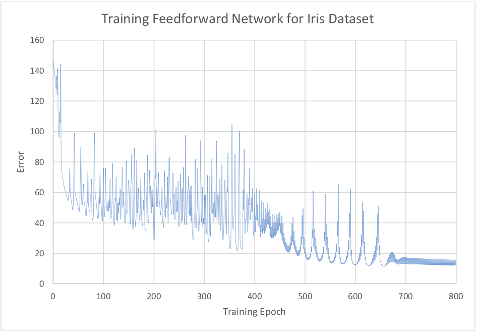
Figure 6: Error while training network on Iris dataset
Stochastic gradient descent
Often, in practice, computing the error and gradient for the entire training set can be very slow and in some cases not possible if the data will not fit entirely in memory. Stochastic gradient descent solves this problem by performing the back-propagation training on small batches of the training set chosen at random.
Randomly chosen batches simulate real-time streaming of data and help to reduce bias in the final trained network (see chapter 7 in [2] for more details on bias and variance in machine learning).
Classification for 3+ classes using stochastic batch training
This time we will again use Fisher’s Iris dataset, but the network will be trained using randomly selected small batches from the training data.
Conclusion
In this white paper we have explored a proof-of-concept implementation of a feedforward network in kdb+. By constructing the model for the network using linear algebra (inputs, outputs and weights represented by matrices) we have shown that an array-processing language is well suited to developing a complex system.
We have shown that multiple types of output functions can be easily applied to the network depending on the desired result. This generalization demonstrates the adaptability of kdb+ to many problems where numerical data can be arranged into lists, arrays or tables.
In the event that there is not enough main memory to carry out the calculations on all the training data in one pass we presented an alternative approach, stochastic gradient descent, which allows the network to be trained on small batches of the data.
The network exhibited in this paper forms the groundwork for more complicated networks. Adding additional hidden layers and different options for threshold function will allow more complex convolutional and deep networks to be developed.
All tests were run using kdb+ version 3.2 (2015.05.07)
Author
James Neill works as a kdb+ consultant for one of the world’s largest investment banks, developing a range of applications. James has also been involved in the design of training courses in data science and machine learning as part of the First Derivatives training programme.
References
-
Murphy, K. P. (2012). Machine Learning: a probabilistic perspective. MIT Press.
-
Hastie, T., Tibshirani, R. and Friedman, J. The Elements of Statistical Learning. Springer, New York. (Online version)
-
Alpaydin, E. Introduction to Machine Learning, Second Edition. MIT Press.