Code profiler

Experimental feature

Currently implemented for x86_64 Linux (kdb+ l64).

kdb+ 4.0 includes an experimental built-in call-stack snapshot primitive that allows building a sampling profiler.

A sampling profiler is a useful tool for low-overhead instrumentation of code performance characteristics. For inspiration, we have looked at tools like Linux perf.

A new function, .Q.prf0, returns a table representing a snapshot of the call stack at the time of the call in another kdb+ process.

Warning

The process to be profiled must be started from the same binary as the one running .Q.prf0, otherwise 'binary mismatch is signalled.

.Q.prf0 stops the target process for the duration of snap-shotting.

Time per call is mostly independent of call-stack depth. You should be able to do at least 100 samples per second with less than 5% impact on target process performance.

The profiler has mostly the same view of the call stack as the debugger. .Q.prf0 returns a table with the following columns:

name    assigned name of the function
file    path to the file containing the definition
line    line number of the definition
col     column offset of the definition, 0-based
text    function definition or source string
pos     execution position (caret) within text

For example, given the following /w/p.q:

.z.i
a:{b x};b:{c x}
c:{while[1;]}
a`

running it with \q /w/p.q, setting pid to the printed value, the following call-stack snapshot is observed (frames corresponding to system and built-in functions can be filtered out with the .Q.fqk predicate on file name):

q)select from .Q.prf0 pid where not .Q.fqk each file
name  file     line col text          pos
-----------------------------------------
""    "/w/p.q" 4    0   "a`"          0
"..a" "/w/p.q" 2    2   "{b x}"       1
"..b" "/w/p.q" 2    10  "{c x}"       1
"..c" "/w/p.q" 3    2   "{while[1;]}" 7

Permissions

By default on most Linux systems, a non-root process can only profile (using ptrace) its direct children.

: Yama documentation

\q starts a child process, so you should be able to profile these with no system changes.

If you wish to profile unrelated processes, you have a few options:

• change kernel.yama.ptrace_scope as detailed in the link above

• give the q binary permission to profile other processes with

  setcap cap_sys_ptrace+ep $QHOME/l64/q

• run the profiling q as root

Docker

To avoid the limitation to direct child processes:

docker run … --cap-add=SYS_PTRACE

Usage

Typically a sampling profiler collects call-stack snapshots at regular intervals. It is convenient to use q’s timer for that:

.z.ts:{0N!.Q.prf0 pid};system"t 10" /100Hz

There are a few toys provided. Their usages follow the same pattern: they accept a single argument, either a script file name to run, or a process ID to which to attach. In the former case, a new q process is started with \q running the specified file. Exit with \\.

top.q

shows an automatically updated display of functions most heavily contributing to the running time (as measured by number of samples in which they appear). self is the percentage of time spent in the function itself; total includes all descendants.

record.q

writes the samples to disk in a splayed table prof, one sample per row.

With prof thus recorded, try

`:prof.txt 0:(exec";"sv'ssr[;"[ ;]";"_"]each'name from`:prof),\:" 1"

to generate prof.txt suitable for feeding into FlameGraph or speedscope for visualization.

Walk-through

Let’s apply the profiler to help us optimize an extremely naïve implementation of Monte-Carlo estimation of π. We'll use record.q and speedscope as described above.

Start with the following /w/pi.q consisting of purely scalar code:

point:{-1+2?2.}
dist:{sqrt sum x*x}
incircle:{1>dist x}
run:{n:0;do[x;n+:incircle point[]];4*n%x}
\t 0N!run 10000000

This takes ~12s on a commodity laptop. Get the profile (running q record.q /w/pi.q), convert to prof.txt and open the result in speedscope. All three tabs offer useful views of the execution profile:

• Time Order presents call stack
• Left Heavy aggregates similar call stacks together, like FlameGraph
• Sandwich shows an execution profile similar to top.q

In this very simple case, Sandwich suffices, but feel free to explore different representations.

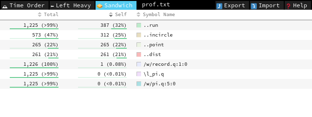
run takes most of the time (Self column), and we can improve it by getting rid of the scalar loop:

run:{4*(sum incircle each point each til x)%x}

This gets us a modest increase in performance, and looking at the profile again:

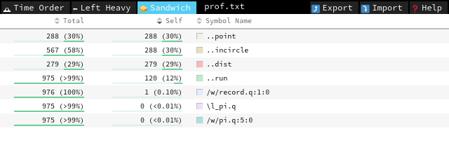
we see that run no longer dominates the profile; now point and incircle do. We note that incircle is already vectorized, so we should focus on getting a better random-point sampling function.

points:{2 0N#-1+(2*x)?2.}
run:{4*(sum incircle points x)%x}

This runs in ~400ms – around a 30× improvement. The rest is left as an exercise for the reader.