Build and backtest scalable trading strategies using real time and historical tick data
Overview
Use kdb Insights Enterprise to stream live with historical tick data to develop interactive analytics; powering faster, and better in-the-moment decision-making.
Benefits
| benefit | description |
|---|---|
| Live and historical view | To maximize opportunity, you need both real time and historical views of your market share. Use kdb Insights Enterprise to stream live tick data alongside historical data for the big picture view of the market. |
| React in real time | React to market events as they happen; not minutes or hours later, to increase market share through efficient execution. |
| Aggregate multiple sources | Aggregate your liquidity sourcing for a better understanding of market depth and trading opportunities. |
Financial dataset
kdb Insights Enterprise lets you work with both live and historical data. This example provides a real-time price feed alongside historical trade data. The real-time price feed calculates two moving averages. A cross between these two moving averages establishes a position (or trade exit) in the market.
1. Build a database
- Select Build a Database under Discover kdb Insights Enterprise of the Overview page.
- Name the database (e.g.
equities), select a database size, typically Starter; click Next. -
Define schema; for small data sets, continue with the Column Input. There is also a JSON Code View option is available for adding large schema tables, found to the top right corner.
-
Define schemas for three data tables named as:
trade,close, andanalytics. Column descriptions are optional and not required here.column type timestamp timestamp price float volume integer column type Date date Time timestamp Open float High float Low float Close float AdjClose float Volume long AssetCode symbol column type timestamp timestamp vwap float twap float open float high float low float close float -
Remove
On-Disk Attributeson each table; by default, these are set on the first column.Expand the first column by clicking the down arrow, set both
On-Disk Attributesto None.setting value On-Disk Attribute (Ordinal Partitioning) None On-Disk Attribute (Temporal Partitioning) None -
Under Essential Properties, review the schema partitions for each table and set them to the following:
setting value Type partitioned Partition Column timestamp setting value Type splayed setting value Type partitioned Partition Column timestamp -
On the same page, open the Advanced Properties accordion and ensure all sort columns are empty; typically, sort columns are assigned to the timestamp column - so just remove them if present.
- Click
-
Replace the JSON in the code editor with:
equities schema
Paste the JSON code into the code editor:
[ { "name": "trade", "type": "partitioned", "primaryKeys": [], "prtnCol": "timestamp", "sortColsDisk": [], "sortColsMem": [], "sortColsOrd": [], "columns": [ { "type": "timestamp", "name": "timestamp", "primaryKey": false, "attrMem": "", "attrOrd": "", "attrDisk": "" }, { "name": "price", "type": "float", "primaryKey": false, "attrMem": "", "attrOrd": "", "attrDisk": "" }, { "name": "volume", "type": "int", "primaryKey": false, "attrMem": "", "attrOrd": "", "attrDisk": "" } ] }, { "name": "close", "columns": [ { "type": "date", "name": "Date", "primaryKey": false, "attrMem": "", "attrOrd": "", "attrDisk": "" }, { "name": "Time", "type": "timestamp", "primaryKey": false, "attrMem": "", "attrOrd": "", "attrDisk": "" }, { "name": "Open", "type": "float", "primaryKey": false, "attrMem": "", "attrOrd": "", "attrDisk": "" }, { "name": "High", "type": "float", "primaryKey": false, "attrMem": "", "attrOrd": "", "attrDisk": "" }, { "name": "Low", "type": "float", "primaryKey": false, "attrMem": "", "attrOrd": "", "attrDisk": "" }, { "name": "Close", "type": "float", "primaryKey": false, "attrMem": "", "attrOrd": "", "attrDisk": "" }, { "name": "AdjClose", "type": "float", "primaryKey": false, "attrMem": "", "attrOrd": "", "attrDisk": "" }, { "name": "Volume", "type": "long", "primaryKey": false, "attrMem": "", "attrOrd": "", "attrDisk": "" }, { "name": "AssetCode", "type": "symbol", "primaryKey": false, "attrMem": "", "attrOrd": "", "attrDisk": "" } ], "type": "splayed", "primaryKeys": [], "sortColsMem": [], "sortColsOrd": [], "sortColsDisk": [] }, { "name": "analytics", "columns": [ { "type": "timestamp", "name": "timestamp", "primaryKey": false, "attrMem": "", "attrOrd": "", "attrDisk": "" }, { "name": "vwap", "type": "float", "primaryKey": false, "attrMem": "", "attrOrd": "", "attrDisk": "" }, { "name": "twap", "type": "float", "primaryKey": false, "attrMem": "", "attrOrd": "", "attrDisk": "" }, { "name": "open", "type": "float", "primaryKey": false, "attrMem": "", "attrOrd": "", "attrDisk": "" }, { "name": "high", "type": "float", "primaryKey": false, "attrMem": "", "attrOrd": "", "attrDisk": "" }, { "name": "low", "type": "float", "primaryKey": false, "attrMem": "", "attrOrd": "", "attrDisk": "" }, { "name": "close", "type": "float", "primaryKey": false, "attrMem": "", "attrOrd": "", "attrDisk": "" } ], "type": "partitioned", "primaryKeys": [], "prtnCol": "timestamp", "sortColsMem": [], "sortColsOrd": [], "sortColsDisk": [] } ] -
Applythe JSON,
-
-
Click Next
- The final step gives a summary of the database; click
 to complete.
 - The database runs through the deployment process; when successful, the database listed in the left-hand menu shows a green tick and is active for use.
Database warnings
Once the database is active you will see some warnings in the Issues pane of the Database Overview page, these are expected and can be ignored.
2. Ingest live data
The live data feed uses Apache Kafka. Apache Kafka is an event streaming platform easily consumed and published by kdb Insights Enterprise.
- Select Import under Discover kdb Insights Enterprise of the Overview page.
-
Select the
Kafkanode and complete the properties;*are required fields:setting value Broker* 34.130.174.118:9091 Topic* spx Offset* End Use TLS* No Use Schema Registry* No -
Click Next.
- Select a decoder. Event data on Kafka is of type JSON; select the
JSONdecoder, then click Next -
Incoming data is converted to a type compatible with a kdb Insights Enterprise database using a schema. The schema is already defined as part of database creation; Click
 . Then select the database created in 1. Build a Database and its
 tradeschema. Data Format is unchanged asAny. Parse Strings is kept asautofor all fields.setting value Data Format* Any -
Click Load to apply the schema.
- Click Next.
-
The Writer step defines the data written to the database. Use the database and table defined in step 1.
setting value Database* Name as defined in 1. Build a database Table* trade Write Direct to HDB Unchecked Deduplicate Stream Enabled -
Click
 to open a view of the pipeline in the pipeline template.
Modify pipeline
The data ingest process finishes with a pipeline view. The Kafka ingest requires one more step, or node, in the pipeline. Use the pipeline template to add the extra step.
Data is converted from an incoming JSON format on the Kafka feed, to a kdb+ friendly dictionary. But the missing step requires a conversion from a kdb+ dictionary to a kdb+ table before deployment. This is done using enlist.
- In the pipeline template, open the Functions node list in the left-hand-menu and click and drag the Map function node into the pipeline teamplate workspace.
- Disconnect the connection between the Decoder and Transform node with a right-click on the join.
-
Insert the Map function between the Decoder and Transform nodes; drag-and-connect the edge points of the Decoder node to the Map node, and from the Map node to the Transform node.
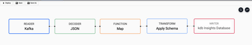
Kakfa pipeline with the inserted Map function node between JSON Decoder node and schema Transform node. -
Update the Map function node by adding to the code editor. You have the choice of using enter either
pythonorqcode:import pandas as pd import pykx as kx def func(data): dataDict = data.pd() vals,keys = list(dataDict.values()), list(dataDict.keys()) newDf = pd.DataFrame(vals,index=keys) return kx.K(newDf.transpose()){[data] enlist data } -
Click
 to save details to the node.
3. Ingest historical data
Where Kafka is used to feed live data to kdb Insights Enterprise, historic data is kept on object storage. Object storage is ideal storage for unstructured data, eliminating the scaling limitations of traditional file storage. Limitless scale makes it the storage of the cloud with Amazon, Google and Microsoft all employing object storage as their primary storage.
Historicaltrade data is maintained on Microsoft Azure Blob Storage.
- Select Import under Discover kdb Insights Enterprise of the Overview page.
-
Select
Microsoft Azure Storageand complete the properties;*are required:setting value Path* ms://kxevg/close_spx.csv Account* kxevg File Mode* Binary Offset* 0 Chunking* Auto Chunk Size* 1MB -
Click Next.
-
Select a decoder. The historic data is stored as a csv file in the cloud; select CSV decoder and complete the properties:
setting value Delimiter , Header First Row Encoding Format UTF8 -
Click Next.
- Next, transform the data into a format compatible with a kdb Insights Enterprise database with a schema. Click . Select the database created in step 1, then chose the
closetable schema. Data Format is unchanged asAny. Parse Strings is kept asautofor all fields. - Click Load to apply the schema.
- Click Next.
-
Define the database to write data too:
setting value Database* Name as defined in 1. Build a database Table* close Write Direct to HDB Unchecked Deduplicate Stream Enabled -
Click
to open a view of the pipeline.
4. Save pipelines
For each ingest pipeline, click Save and give the pipeline a name. Saved pipelines are listed under the Pipelines menu of the Overview page.
5. Deploy pipelines
Select each of the pipelines and deploy them. This activates the pipeline, making the data available for use.
Deployed pipelines are listed under Running Pipelines of the Overview page. When the first pipeline reaches a Status=Running, and the second reaches a Status=Finished, then the data is loaded.
6. Query the data
Data queries are run in the query tab; this is accessible from the [+] of the ribbon menu, or Query under Discover kdb Insights Enterprise of the Overview page.
- Select the
SQLtab of the query page. -
To retrieve a count of streaming events in the
tradetable, add to the code editor:SELECT COUNT(*) FROM trade -
Define an Output Variable - this is required.
-
Click
 to execute the query. Rerun the query to get an updated value.
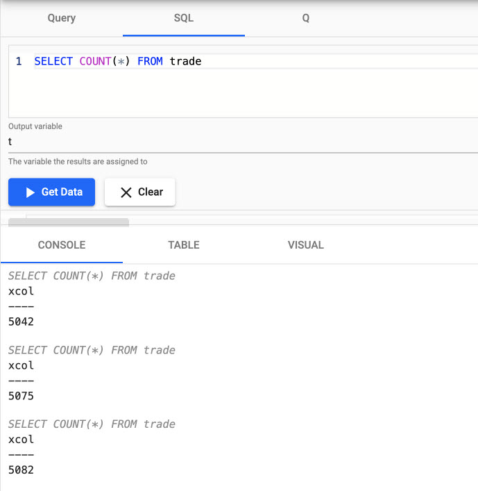
ASQLquery reporting the count of trade events from the Kafka feed. -
Right-click in the Console to clear the results.
-
In the
SQLtab, replace the existing code with:SELECT * FROM close -
Define an Output Variable
-
Click
to execute the query.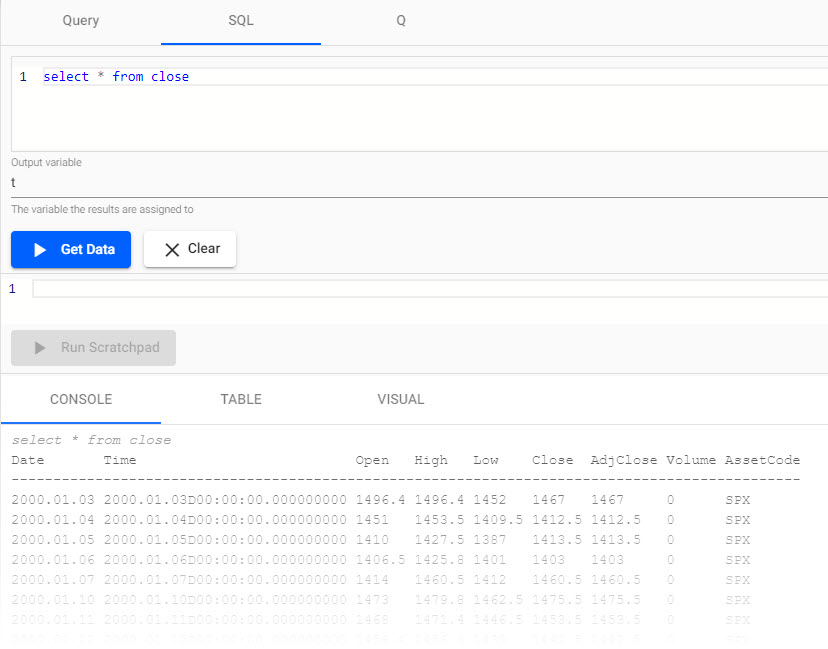
ASQLquery reporting end-of-day S&P historic prices.
7. Create powerful analytics
Using the data, a trade signal is created to generate a position in the market (S&P).
In the SQL query tab, run (against Kafka pipeline data):
SELECT * FROM trade
In the output, toggle between console, table or chart for different views of the data; for example, a chart of prices over time.
A SQL query against streaming trade data, viewed in the console, as a table, or a time series chart.
Long and short position simple moving averages
The strategy calculates two simple moving averages; a "fast", short time period moving average, and a "slow", long time period moving average.
When the "fast" line crosses above the "slow" line, we get a 'buy' trade signal, with a 'sell' signal on the reverse cross.
This strategy is also an "always-in-the-market" signal, so when a signal occurs, it not only exits the previous trade, but opens a new trade in the other direction; going long (buy low - sell high) or short (sell high - buy back low) when the "fast" line crosses above or below the "slow" line.
Create a variable analytics in the scratchpad to calculate the "fast" and "slow" moving average:
// taking the close price we calculate two moving averages:
// 1) shortMavg on a window of 10 sec and
// 2) longMavg on a window of 60
analytics : select timestamp,
                   price,
                   shortMavg:mavg[10;price],
                   longMavg:mavg[60;price]
                from t
This strategy uses a 10-period moving average for the "fast" signal, and a 60-period moving average for "slow" signal. Streamed updates for the moving average calculations are added to the chart.
A "fast" and "slow" moving average zoomed in the visual chart view.
Trade position
The crossover of the two "fast" and "slow" moving averages creates trades. These will be tracked with a new variable called positions.
In the scratchpad, add:
// when shortMavg and long Mavg cross each other we create the position
// 1) +1 to indicate the signal to buy the asset or
// 2) -1 to indicate the signal to sell the asset
positions : select timestamp,
                   position:?[shortMavg<longMavg;-1;1],
                   return:log[price % prev price]
                from analytics
q/kdb+ functions explained
If any of the above code is new to you don't worry, we have detailed the q functions used above:
- ?[x;y;z] when x is true return y, otherwise return z
- x<y returns true when x is less than y, otherwise return false
- log to return the natual logarithm
- x%y divides x by y
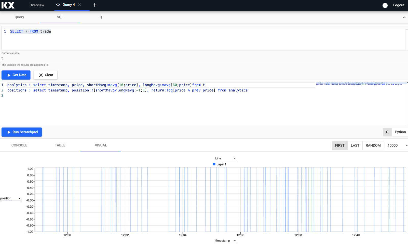
A position analytic to track crossovers between the "fast" and "slow" moving averages; signals displayed in the query visual chart.
Active vs. passive strategy
The current, active strategy is compared to a passive strategy; i.e. a strategy tracking a major index, like the S&P 500 or a basket of stocks, such as an ETF. We want to know if our strategy performs better.
Read more about active and passive strategies
In scratchpad, we create a new variable called performance to generate a benchmark to compare strategy performance too.
performance : select timestamp,
                     benchmark: exp sums return,
                     strategy: exp sums return * prev position
                from positions
q/kdb+ functions explained
If any of the above code is new to you don't worry, we have detailed the q functions used above:
- exp raise e to a power where e is the base of natual logarithms
- sums calculates the cumulative sum
- * to multiply
- prev returns the previous item in a list
The result is plotted on a chart. The active strategy outperforms the passive benchmark.
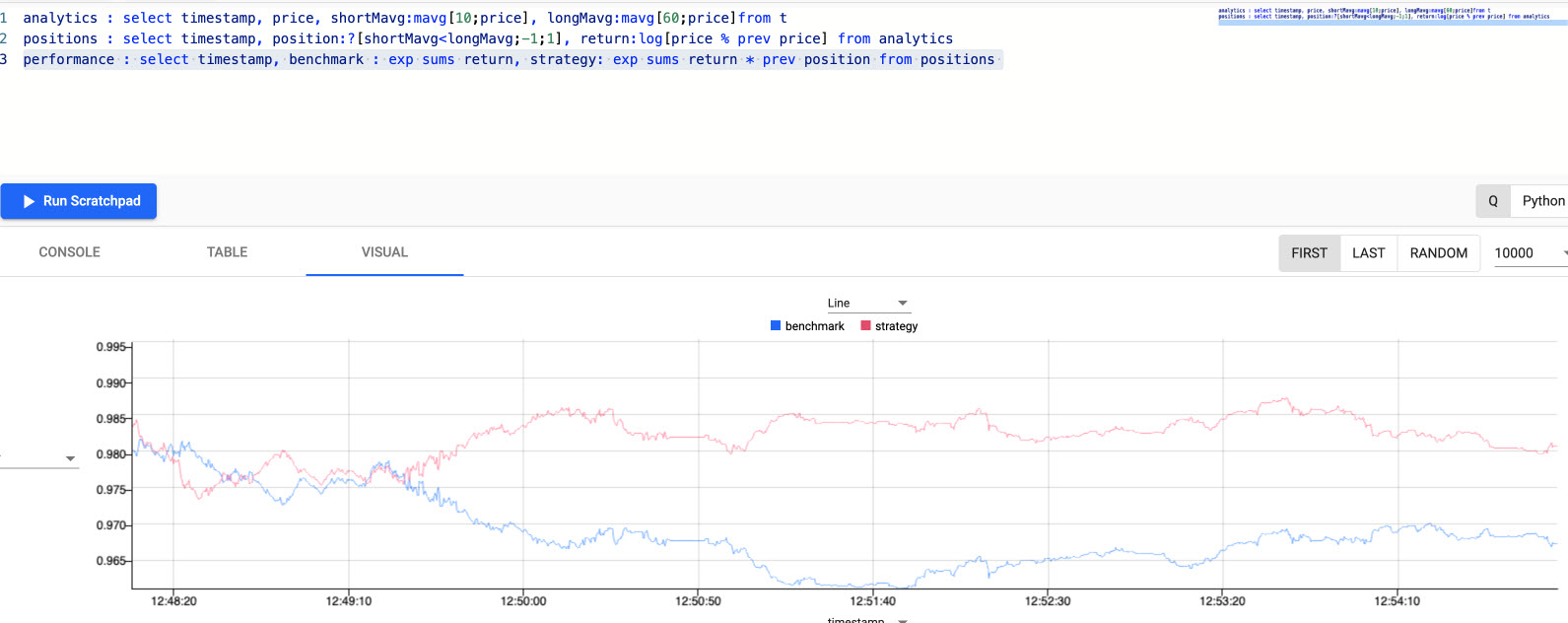
The active moving average crossover strategy is compared to a passive benchmark; the strategy outperforms the benchmark as illustrated in the chart.
8. Create a dashboard view
Up to now, ad hoc comparative analysis was conducted in the scratchpad. We can formalize this better by creating a dashboard view.
A view can be opened from the [+] ribbon menu, or selecting Visualize under Discover kdb Insights Enterprise of the Overview page.
Views only use data persisted in a database
Views can only access data stored on an active database. All analytic outputs must be saved to the database.
Persisting analytics
The quickest way to persist an analytic is to modify the data pipeline used by the analytic.
Open the Kafka pipeline template; select it from the left-hand pipeline menu of the Overview page.
-
From the pipeline template view, add a Function Split node from the list of nodes. Position it between the Function Map node and the Transform Apply Schema node; right-click existing links to clear, before reconnecting the point-edges with a drag-and-connect. This will leave one available point-edge in the Split node.
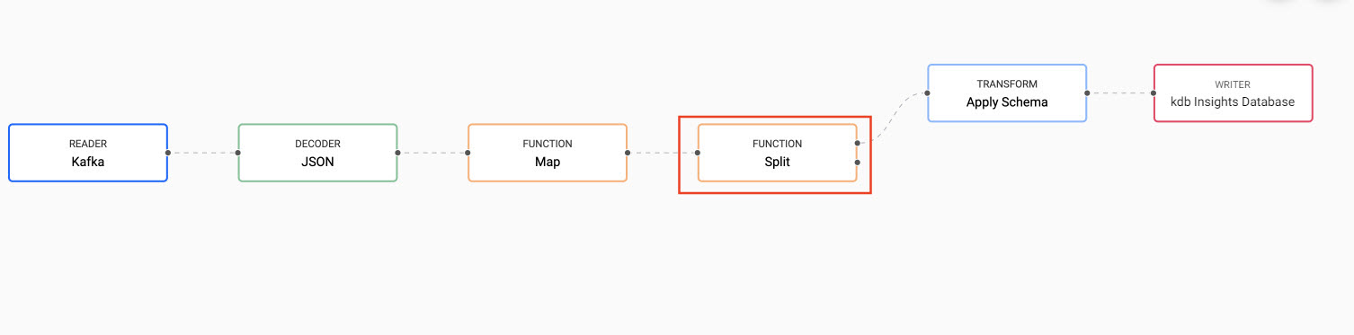
The Function Split node positioned between the Function Map node and the Transform schema node; drag-and-connect the edge points of a node to reconnect pipeline nodes. -
Add a Window Timer Window to the pipeline workspace. Connect it to the second point-edge of the Function Split node. The Timer Window aggregates incoming data by time. Set the timer to run every 5 seconds;
*are required properties. Apply changes.property value Period 0D00:00:05 Skip empty windows* Unchecked Use Count Triggger* Uncecked 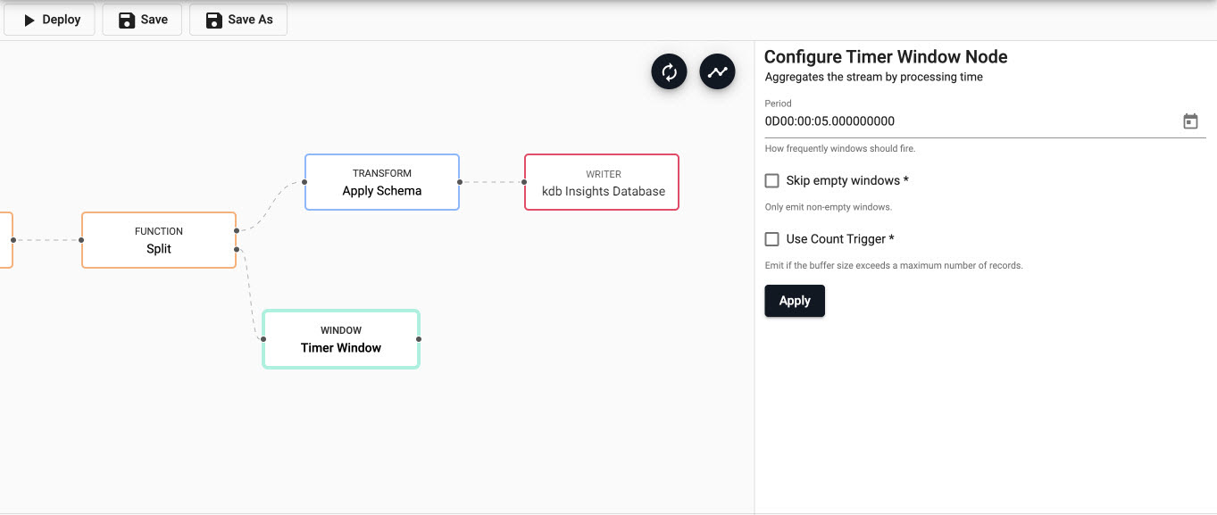
The Window Timer Window is configured to fire every 5 seconds. Connect to the Function Split node. -
We define the business logic for the analytic in a Function Map node. Add a Function Map node and connect it to the Window Timer Window. In the code editor, add - then apply:
// the following code is calculating the fields:
// 1) vwap = weighted average price, adjusted by volume, over a given time period
// 2) twap = weighted average price over a given time period
// 3) open = price at which a security first trades when an exchange opens for the day
// 4) high = highest price security is traded at
// 5) low = lowest price security is traded at
// 6) close = price at which a security last trades when an exchange closes for the day
// 7) volume = volume of trades places
{[data]
    select last timestamp,
       vwap:|[1;volume] wavg price,
       twap:last[price]^(next[timestamp]-timestamp) wavg price,
       open:first price,
       high:max price,
       low:min price,
       close: last price
    from update "P"$timestamp,
         volume:|[1;volume]
    from data
    }
kdb+/q functions explained
If any of the above code is new to you don't worry, we have detailed the q functions used above:
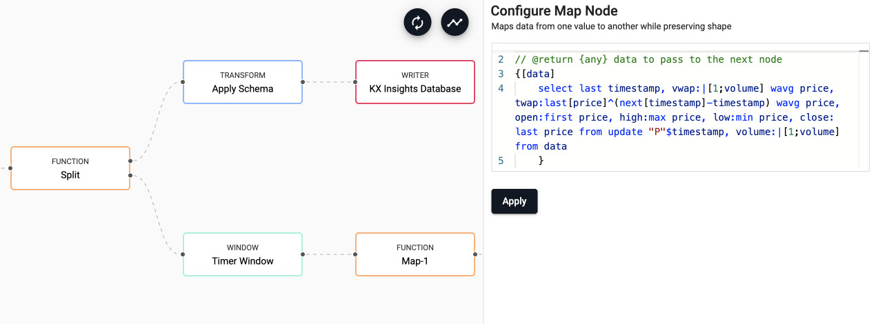
The Function Map node contains the business logic for the analytic. This is connected to the Window Timer Window in the pipeline. -
The data generated by the analytic has to be transformed and written to the database. The steps are the same as for the kafka pipeline, except the
analyticstable should be used in place ofclosefor the schema and writing to database.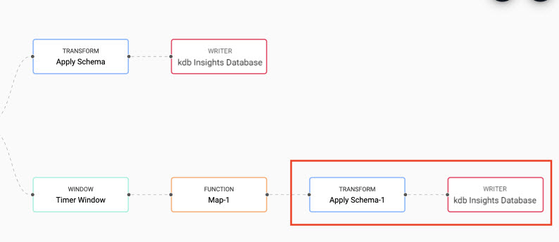
Connect a Transform Apply Schema and Writer _KX Insights Database node to the Function Map node by the analytic. Ensure theanalyticstable is used for both the Transform and Writer node._ -
Save the modified Kafka pipeline.
- Deploy the modified Kafka pipeline. A successful deployment shows
Status=Runningunder Running Pipelines of the Overview page.
Load and review the ready-made report
- Create a new Report by selecting the plus icon at the top toolbar and select Report.
- Download the completed report Equities.json and drop it into this new blank Report.
Note that the dashboard has two screens.
The first "Chart" view uses both live and historic data for the big picture in the market.
The top chart in the dashboard plots the price data and VWAP analytic generated by the Kafka pipeline.
The lower chart plots historic index data ingested by the Azure object storage pipeline.
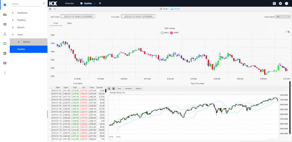
Access the Equities view from the left-hand menu of the Overview page. The top chart is a live feed of price and the calculated VWAP analytic. The lower chart is a time series chart of historic index data.
The second "Table" dashboard view tracks positions in the market.
In the top chart, a green highlight is used if a Long (a buyer) trade, or red if Short (a seller).
A similar highlight is used in the table on the left and in the volume bars of the lower chart.
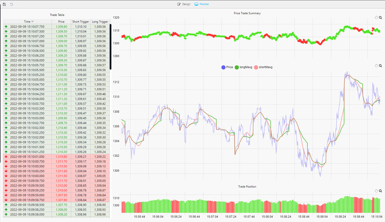
The Chart view shows the strategy position in the market; long trades are marked in green and short trades in red.
I want to learn more building views
What's next?
Learn how to build and run a machine learning model to create stock predictions in real-time on this financial dataset in the next tutorial.