Integrate Kafka and kdb+ for real-time telemetry
This dashoard view monitors NYC subway train punctuality for travel planning.
Overview
Real-time information on train times is a Apache Kafka feed.
Real-time data can be seamlessly handled in kdb Insights Enterprise using pipelines connecting to data sources. Apache Kafka is an event streaming platform that can be easily published to and consumed by kdb Insights Enterprise.
Guided walkthrough
Requires an insights-demo database. Available databases are listed under Databases in the Overview page; create an insights-demo database if none available.
Benefits
| benefit | description |
|---|---|
| Get a Live View | Use kdb Insights Enterprise to stream data from Kafka for a continuous view of your transactional data. |
| Real Time Monitoring | View business events as they happen; be responsive not reactive. |
| Get Analytics-Ready Data | Get your data ready for analytics before it lands in the cloud. |
Subway dataset
Kdb Insights Enterprise helps you easily consume Kafka natively. A real time demo of NYC subway dataset is available with Kafka, offering live alerts for NYC subway trains including arrival time, stop location coordinates, direction and route details.
1. Build a database
- Select Build a Database under Discover kdb Insights Enterprise of the Overview page.
- Name the database (e.g.
insights-demo), select a database size, typically Starter; click Next. -
Define a schema for a
subwaytable. Column descriptions are optional and not required here.Subway schema
column type trip_id symbol arrival_time timestamp stop_id symbol stop_sequence short stop_name symbol stop_lat float stop_lon float route_id short trip_headsign symbol direction_id symbol route_short_name symbol route_long_name symbol route_desc string route_type short route_url symbol route_color symbol -
In Essential Properties, set
Partition Columntoarrival_time. - Open Advanced Properties accordion and ensure all sort columns are empty; typically, sort columns are assigned to the timestamp column - so just remove them if present.
- Click Next.
- The final step gives a summary of the database; click
 to complete.
 - The database runs through the deployment process; when successful, the database listed in the left-hand menu shows a green tick and is active for use.
Database warnings
Once the database is active you will see some warnings in the Issues pane of the Database Overview page, these are expected and can be ignored.
2. Ingest live Data
The subway feed uses Apache Kafka. Apache Kafka is an event streaming platform easily consumed and published by kdb Insights Enterprise.
- Select Import under Discover kdb Insights Enterprise of the Overview page.
-
Select the
Kafkanode and complete the properties;*are required fields:setting value Broker* 34.130.174.118:9091 Topic* subway Offset* End Use TLS disabled -
Click Next.
- Select a decoder. Event data on Kafka is of type JSON; select the
JSONdecoder, then click Next -
Incoming data is converted to a type compatible with a kdb Insights Enterprise database using a schema. The schema is already defined as part of database creation; Click
 . Then select the database created in 1. Build a Database and the
 subwayschema. Data Format is unchanged asAny. Parse Strings is kept asautofor all fields.setting value Data Format* Any Guided walkthrough
Select the
insights-demodatabase to get thesubwayschema. -
Click Load to apply the schema.
- Click Next.
-
The Writer step defines the data write to database. Use the database and table defined in step 1.
setting value Database* Name as defined in 1. Build a database Table* subway Write Direct to HDB Unchecked Deduplicate Stream Enabled -
Click
 to open a view of the pipeline in the pipeline template.
Modify Pipeline
The data ingest process finishes with a pipeline view. The Kafka ingest requires one more step, or node, in the pipeline. Use the pipeline template to add the extra step.
Data is converted from an incoming JSON format on the Kafka feed, to a kdb+ friendly dictionary. But the missing step requires a conversion from a kdb+ dictionary to a kdb+ table before deployment. This is done using enlist.
- In the pipeline template, open the Functions node list in the left-hand-menu and click and drag the Map function node into the pipeline template workspace.
- Disconnect the connection between the Decoder and Transform node with a right-click on the join.
-
Insert the Map function between the Decoder and Transform nodes; drag-and-connect the edge points of the Decoder node to the Map node, and from the Map node to the Transform node.
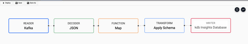
Kakfa pipeline with the inserted Map function node between JSON Decoder node and schema Transform node. -
Update the Map function node by adding to the code editor:
5. Click{[data] enlist data } to save details to the node.
3. Save pipeline
Save and name the pipeline (subway). Saved pipelines are listed under the Pipelines menu of the Overview page.
4. Deploy pipeline
Select and deploy the pipeline. This activates the pipeline, making the data available for use.
Deployed pipelines are listed under Running Pipelines of the Overview page. The subway pipeline reaches Status=Running when data is loaded.
5. Query the data
Kafka event count
Data queries are run in the query tab; this is accessible from the [+] of the ribbon menu, or Query under Discover kdb Insights Enterprise of the Overview page.
- Select the
SQLtab of the query page. -
To retrieve a count of streaming events in the
subwaytable, use the query:SELECT COUNT(*) FROM subway -
Define an Output Variable - this is required.
-
Click
 to execute the query. Rerun the query to get an updated value.
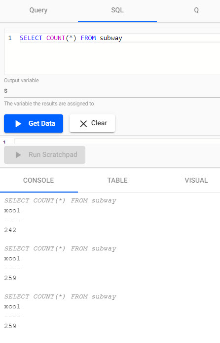
ASQLquery reporting a count of events from the Kafka feed.
Filtering and visualizing
Next, get a subset of the data and save it to an output variable, s.
Set today's date in q
Use .z.d as a convienient way to return today's date.
- In the
qtab, select theinsights-demoand theidbinstance. -
Use the query
3. Define the Output Variable asselect from subway where arrival_time.date in .z.ds. 4. Click to execute the query.
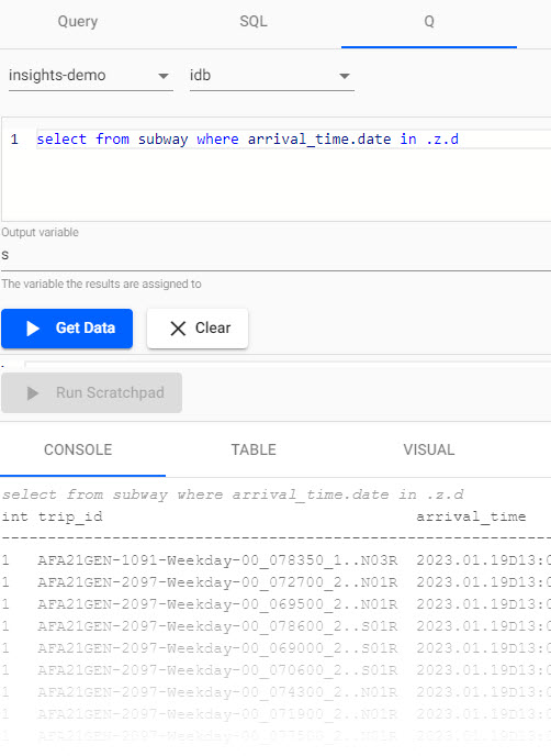
Aqquery listing arrival time of trains for today. -
Additional analysis can be done against the
svariable of today's train data with the scratchpad. Querying in the scratchpad is more efficient than direct querying of the database and supports bothqandpython. Pull data for a selectedtrip_id; change the value of thetrip_idto another if the following example returns no results:select from s where trip_id like "AFA21GEN-1091-Weekday-00_033450_1..N03R" -
Click

-
View the result in one of the Console, Table or Visual tabs; note, you have to rerun the query for each tab change.
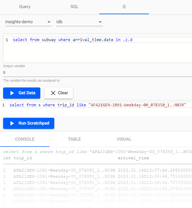
Aqquery run in scratchpad for a selected trip. -
In the Visual inspector, set the y-axis to use
stop_sequenceand x-axis toarrival_timereturns a plot of journey time between each of the stops.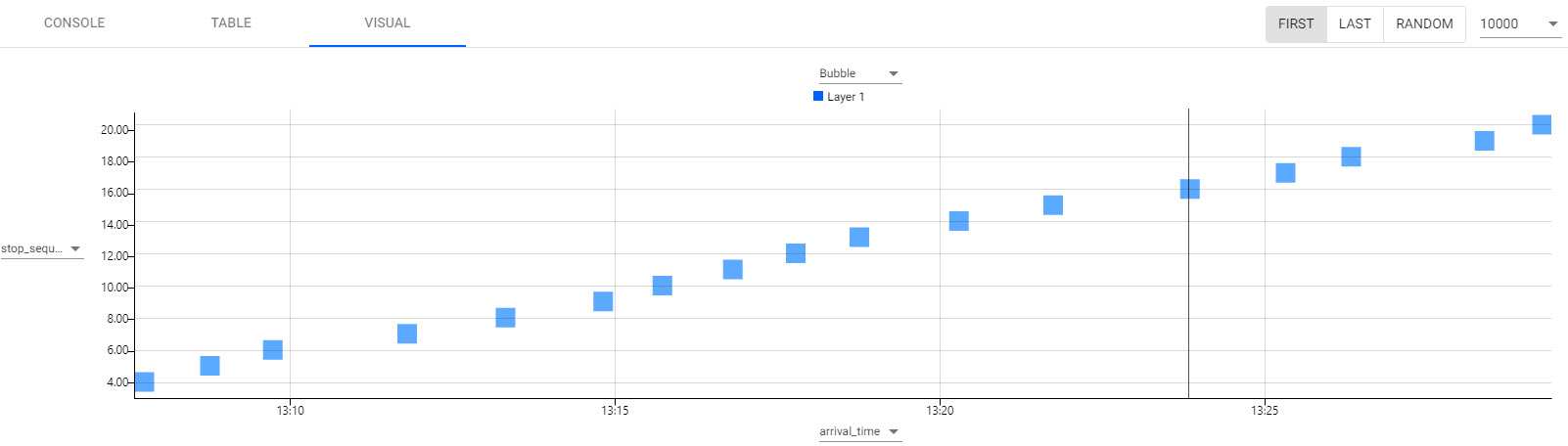
A visual representation of a single trip between each station.
Calculate average time between stops
Calculate the average time between stops as a baseline to determine percentage lateness.
Run in the scratchpad using a trip_id from the previous step; each id is unique:
`arrival_time`time_between_stops xcols
    update time_between_stops:0^`second$arrival_time[i]-arrival_time[i-1] from
    select from s
    where trip_id like "AFA21GEN-1091-Weekday-00_138900_1..N03R"
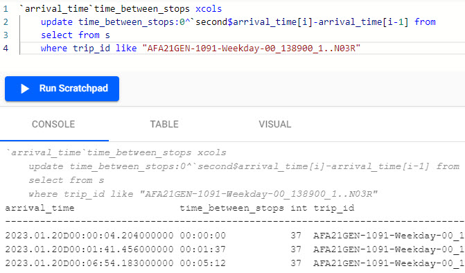
q for calculating average time between stops run in the scratchpad.
New to the q language?
In the above query, the following q elements are used:
- xcols to reorder table columns
- ^ to replace nulls with zeros
- $ to cast back to second datatype
- x[i]-x[i-1] to subract each column from the previous one
If you run into an error on execution, check to ensure the correct code indentation is applied for s3.
What was the longest and shortest stop for this trip?
We can use the Table tab to filter the results - remember to run the scratchpad again on a tab change; for example, doing a column sort by clicking on the column header for the newly created variable time_between_stops will toggle the longest and shortest stop for the selected trip.
Calculating percentage lateness for all trains
Which trains were most frequently on time?
Focus is on trains that completed their entire route. Remove the previous code block, then run in the scratchpad
// Getting the length of each train journey and num of stops
s3:select start_time:first arrival_time,
    journey_time:`second$last arrival_time-first arrival_time,
    first_stop:first stop_name,
    last_stop:last stop_name,
    numstops:count stop_sequence
    by route_short_name,direction_id,trip_id
    from s;
// Filtering only only trains that fully completed their route
s4:select from s3 where numstops=(max;numstops) fby route_short_name;
// Calculating the average journey time per sroute
s5:update avg_time:`second$avg journey_time by route_short_name from s4;
// Calculating the % difference between actual journey time and average time per route
s6:update avg_vs_actual_pc:100*(journey_time-avg_time)%avg_time from s5
New to the q language?
In the above query, the following q elements are used:
- first, last to get first or last record
- - to subract one column from another
- count to return the number of records
- by to group the results of table by column/s - similar to excel pivot
- fby to filter results by a newly calculated field without needing to add it to table
- x=(max;x) to filter any records that equal the maximum value for that column
- $ to cast back to second datatype
- * to perform multiplication
- % to perform division.
If you run into an error on execution, check to ensure the correct code indentation is applied.
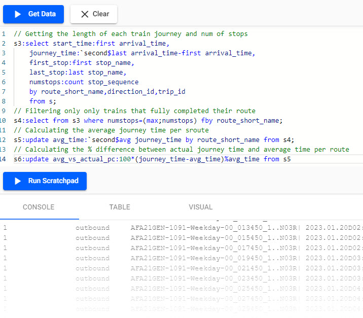
q code for calcuating average journey time.
Most punctual train
Which train was most punctual? Remove the previous code block and then run in the scratchpad
select from s6 where avg_vs_actual_pc=min avg_vs_actual_pc
Using min, the 04:53 route E train was the most punctual (your result will differ).
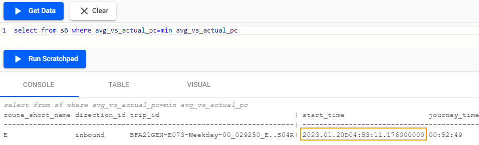
The console shows which train was the most punctual from the Kafka data.
Visualize journey time
Switch to the Visual tab.
Visualize for a single route; remove the previous code block in scratchpad and run
// Filtering for at only inbound trains on Route 1
select from s6 where route_short_name=`1 ,direction_id=`inbound
Switch to a bar chart. Set the y-axis to avg_vs_actual_pc and the x-axis to start_time
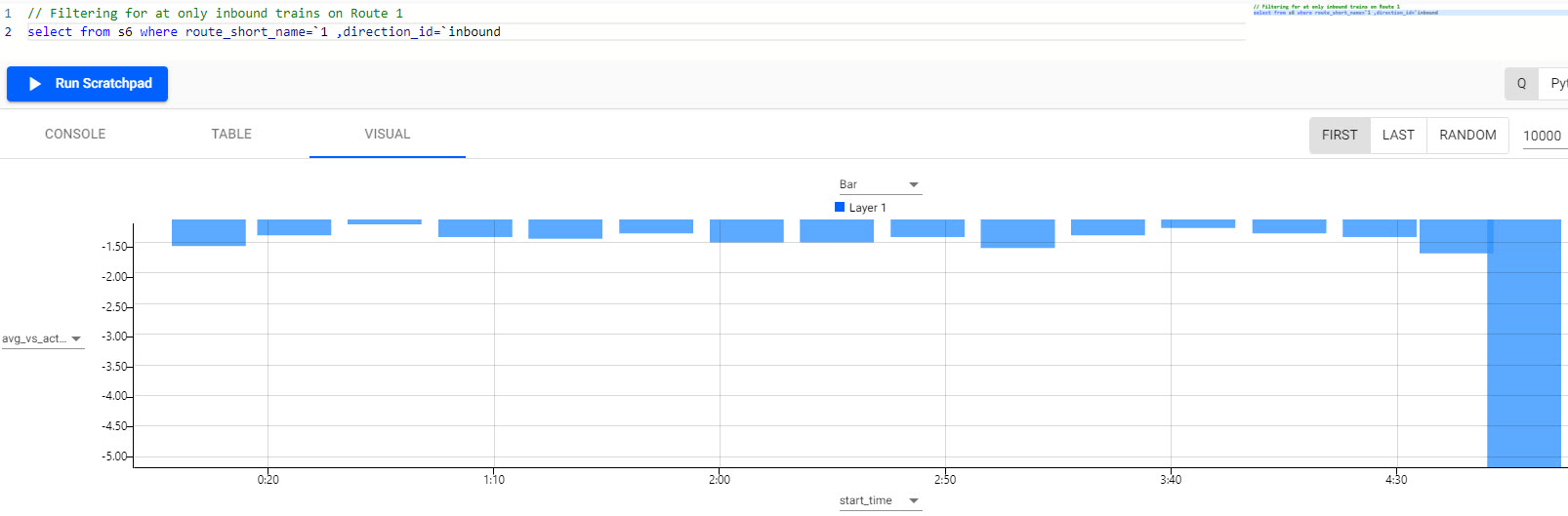
Visualizing the differential between actual and average journey time for a selected route.
Distribution of journey times between stations
Clear the previous code block in scratchpad and run:
{count each group 1 xbar x} 1e-9*"j"$raze exec 1_deltas arrival_time by trip_id from s
From the histogram, the most common journey time between stations is 90 seconds.
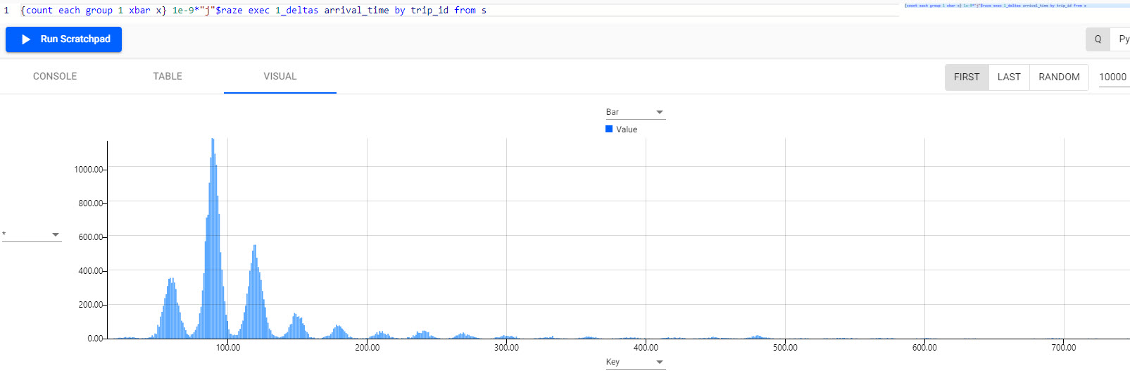
Distribution of journey time between stations. Note peaks at 60, 90, 120, and 150 seconds, with 90 seconds the most common journey time.