Run machine learning model to create stock predictions in real-time
Overview
Use kdb Insights Enterprise to define and run a machine learning model to predict the future state of stock prices.
Ensure you have completed the previous stage first, if not find it here.
Note
This tutorial is to show how you can train a Python-first ML model in the kdb Insights Enterprise platform rather than focusing on developing a particulary accurate model.
Benefits
| benefit | description |
|---|---|
| Python based analysis | Stage data for Python-based analysis to predict future values, such as Neural Network algorithms. |
| ANSI SQL support | Execute using ANSI SQL queries which most Data Science and Machine Leaning tools are familiar. |
| Multiple visualization options | Use the scratchpad to verify the training/test sets and predictions and then move to advanced visualization using Reports or Common BI tools like PowerBi or Tableau to show live data, more depth to the model and empower larger teams to visualize insights. |
Prerequisites
You will need to complete steps 1-2 in the Backtest trading strategies tutorial to ingest the required financial trade table.
Run model
Query dataset
Query the trade data you created in the prerequisites step to get it in the form required for the model later on.
- Select the
SQLtab of the query page. -
To retrieve the open, high, low, close (OHLC) of events in the
tradetable, add this to the code editor:SELECT date_trunc('minute', timestamp) timestamp, FIRST(price) o, MAX(price) h, MIN(price) l, LAST(price) c FROM trade GROUP BY date_trunc('minute', timestamp) -
Define an output variable
ohlc. - Switch window at the bottom of the page from Console to Visual.
-
Click
 to execute the query.
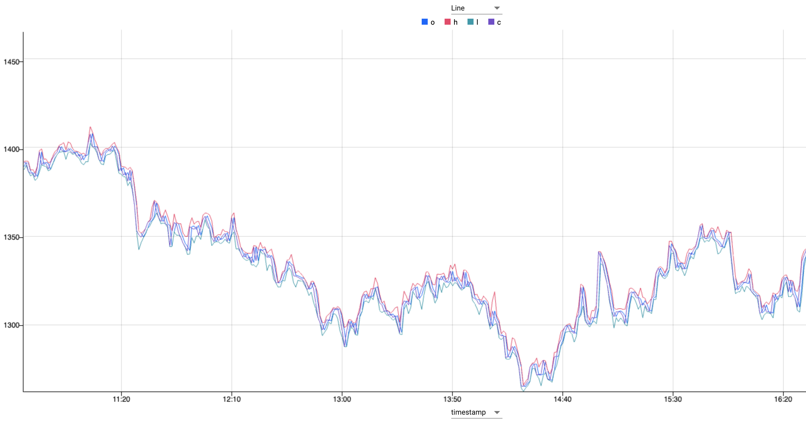
ASQLquery showing open, high, low, close values from the trade table.What does this show?
This OHLC chart shows the open, high, low and closing prices for each period.
OHLC charts are useful since they show the four major data points over a period, with the closing price being considered the most important by many traders.
Run the ML code
For processing the data, a paper written in 2020 used an Long Short-Term Memory algorithm to predict stock prices. Using an open source Git repo, a LTSM model written in Python can be run against the data, to create predictions, and visualize in Scratchpad.
For this section you use the scratchpad for running machine learning model in real-time. The Scratchpad is the middle window of the Query page.
-
In Scratchpad, select
Python. Add the followingPythoncode to the scratchpad editor:Machine Learning Python Code
Paste the following Python code into the scratchpad:
# Imports import pandas as pd import numpy as np import math # Machine learning lib - used here for data preprocessing and calcualtions - applies the range wiht minmaxclater zero and 1 from sklearn.preprocessing import MinMaxScaler # Gets the stat that informs the quality of the prediction from sklearn.metrics import mean_squared_error # Define a neural network model - this is what is being used to predict the future state of the prices later on from keras.models import Sequential from keras.layers import Dense, Activation from keras.layers import LSTM # Reference to the docs -- https://en.wikipedia.org/wiki/Long_short-term_memory # Convert the dataset into dataframe and get averages df = pd.DataFrame (ohlc.pd()) # Axis 1 is horizontal and we want to see this data tabularised OHLC_avg = df[['o','h','l','c']].mean(axis=1) # Preparation of the time series dataset # reshape data preparation step so the data will fit the model applied OHLC_avg = np.reshape(OHLC_avg.values, (len(OHLC_avg),1)) # creates the scaler function scaler = MinMaxScaler(feature_range=(0,1)) # which is applied here OHLC_avg = scaler.fit_transform(OHLC_avg) # Train-test split # Model is trained using 75% of the data - subsample of the data - note that this is the first 75% train_OHLC = int(len(OHLC_avg) * 0.75) # Test data is the remaning 25% so between test and train the whole 100% test_OHLC = len(OHLC_avg) - train_OHLC train_OHLC, test_OHLC = OHLC_avg[0:train_OHLC,:], OHLC_avg[train_OHLC:len(OHLC_avg),:] def new_dataset(dataset, step_size): data_X, data_Y = [],[] for i in range(len(dataset)-step_size-1): a = dataset[i:(i + step_size),0] data_X.append(a) data_Y.append(dataset[i + step_size,0]) # This produces the dataset which tells you what T+1 is within the time-series and organises the data in to what will be used as the features # This feeds the model, and target, which is what is produced return np.array(data_X),np.array(data_Y) # Time-series dataset (for time T, values for time T+1) trainX, trainY = new_dataset(train_OHLC,1) # This give you T which is what you have, and T+1 which the prediction testX, testY = new_dataset(test_OHLC,1) # Reshaping train and test data trainX = np.reshape(trainX, (trainX.shape[0],1,trainX.shape[1])) testX = np.reshape(testX, (testX.shape[0],1,testX.shape[1])) # Gets data into the format that is needed step_size = 1 # LSTM model model = Sequential() model.add(LSTM(32, input_shape=(1,step_size), return_sequences =True)) model.add(LSTM(16)) model.add(Dense(1)) # Beyond the scope of this - takes the features T and learn how to predict what T+1 is model.add(Activation('linear')) # Model compiling and training # compile builds the model into an executable who we will calculate performance and how it is optimised model.compile(loss='mean_squared_error',optimizer='adam') model.fit(trainX, trainY, epochs=5, batch_size=1, verbose=2) # takes the training data fits the model to it that will be used for predictions. # Prediction trainPredict = model.predict(trainX) testPredict = model.predict(testX) # does this # Denormalising and plotting trainPredict = scaler.inverse_transform(trainPredict) trainY = scaler.inverse_transform([trainY]) testPredict = scaler.inverse_transform(testPredict) # Previously the data was weighted artificially with the MinMaxScaler, but that is not a real number for output or for a decision. # This must be now reversed so that the output is actual price data unweighted testY = scaler.inverse_transform([testY]) # Training RMSE trainScore = math.sqrt(mean_squared_error(trainY[0], trainPredict[:,0])) # Calculating how well the predictions match reality trainScore # Test RMSE testScore = math.sqrt(mean_squared_error(testY[0], testPredict[:,0])) # Calculating how well the predictions match reality testScore # Creating similar dataset to plot training predictions trainPredictPlot = np.empty_like(OHLC_avg) trainPredictPlot[:,:] = np.nan # More processing to shape the data for the flattening step trainPredictPlot[step_size:len(trainPredict)+step_size, :] = trainPredict # Creating similar dataset to plot test predictions testPredictPlot = np.empty_like(OHLC_avg) testPredictPlot[:,:] = np.nan # More processing to shape the data for the flattening step testPredictPlot[len(trainPredict)+(step_size*2)+1:len(OHLC_avg)-1, :] = testPredict OHLC_avg = scaler.inverse_transform(OHLC_avg) dataset = pd.DataFrame({ 'tradetime':df['timestamp'] # x axis ,'ohlc': OHLC_avg.flatten() ,'train': trainPredictPlot.flatten() ,'test': testPredictPlot.flatten() }, columns=['tradetime','ohlc','train','test']) dataset -
In the Visual tab, switch the chart type to
Line. -
Run Scratchpad
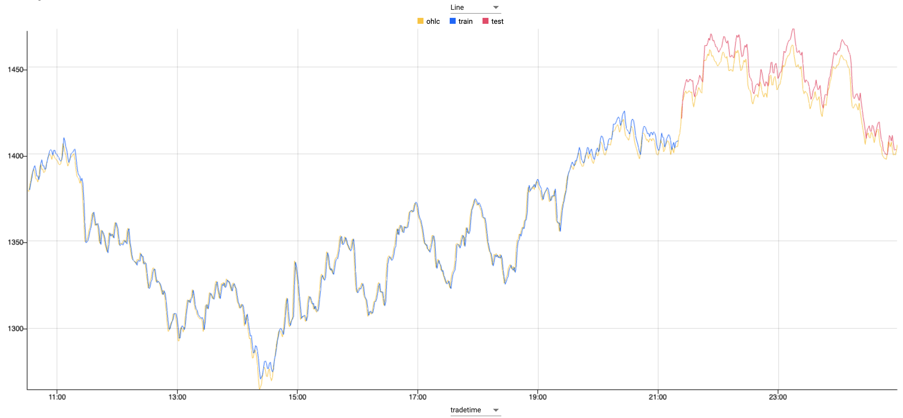
Plot of train, test and predictions datasetWhat is the model doing?
Using standard machine learning libraries that are available in kdb Insights Enterprise the dataset is weighted, shaped and plotted.
The model is first trained using 75% of the data, with the remaining 25% is used to test the model.
Zooming in on the graph where the color changes, you can see where the test dataset begins. Against this test data the predictions follow the live data extremely closely.
What's next?
- Learn how to deploy a machine learning model in a real-time pipeline in the Industry Tutorial.