Apply deep neural networks to streaming IoT data using MQTT and Tensorflow
For manufacturers, machine downtime can cost millions of dollars a year in lost profits, repair costs, and lost production time for employees. By embedding predictive analytics in applications, manufacturing managers can monitor the condition and performance of assets and predict failures before they happen.
kdb Insights Enterprise exists to be the premier cloud-native platform for actionable, data-driven insights.
In this use case, compute logic is applied to live data streaming from a MQTT messaging service. Then Deep Neural Network Regression is used to determine the likelihood of breakdowns.
Benefits
| benefit | description |
|---|---|
| Predictive analysis | Use predictive analytics and data visualizations to forecast a view of asset health and reliability performance. |
| Reduce risks | Leverage data in real time for detection of issues with processes and equipment, reducing costs and maximizing efficiencies throughout the supply chain with less overhead and risk. |
| Control logic | Explore how to rapidly develop and visualize computations to extract insights from live streaming data. |
1: Build a database
- Select Build a Database under Discover kdb Insights Enterprise of the Overview page.
- Name the database (e.g.
manufacturing), select a database size, typically Starter; click Next. - Click
 on the top right hand corner.
 -
Replace the JSON into the code editor
Manufacturing JSON schema
Paste into the code editor:
[ { "name": "sensors", "type": "partitioned", "primaryKeys": [], "prtnCol": "time", "sortColsDisk": [ "time" ], "sortColsMem": [ "time" ], "sortColsOrd": [ "time" ], "columns": [ { "type": "timestamp", "attrDisk": "parted", "attrOrd": "parted", "name": "time", "primaryKey": false, "attrMem": "" }, { "name": "flowplant", "type": "float", "primaryKey": false, "attrMem": "", "attrOrd": "", "attrDisk": "" }, { "name": "pressplant", "type": "float", "primaryKey": false, "attrMem": "", "attrOrd": "", "attrDisk": "" }, { "name": "tempplantin", "type": "float", "primaryKey": false, "attrMem": "", "attrOrd": "", "attrDisk": "" }, { "name": "tempplantout", "type": "float", "primaryKey": false, "attrMem": "", "attrOrd": "", "attrDisk": "" }, { "name": "massprecryst", "type": "float", "primaryKey": false, "attrMem": "", "attrOrd": "", "attrDisk": "" }, { "name": "tempprecryst", "type": "float", "primaryKey": false, "attrMem": "", "attrOrd": "", "attrDisk": "" }, { "name": "masscryst1", "type": "float", "primaryKey": false, "attrMem": "", "attrOrd": "", "attrDisk": "" }, { "name": "masscryst2", "type": "float", "primaryKey": false, "attrMem": "", "attrOrd": "", "attrDisk": "" }, { "name": "masscryst3", "type": "float", "primaryKey": false, "attrMem": "", "attrOrd": "", "attrDisk": "" }, { "name": "masscryst4", "type": "float", "primaryKey": false, "attrMem": "", "attrOrd": "", "attrDisk": "" }, { "name": "masscryst5", "type": "float", "primaryKey": false, "attrMem": "", "attrOrd": "", "attrDisk": "" }, { "name": "tempcryst1", "type": "float", "primaryKey": false, "attrMem": "", "attrOrd": "", "attrDisk": "" }, { "name": "tempcryst2", "type": "float", "primaryKey": false, "attrMem": "", "attrOrd": "", "attrDisk": "" }, { "name": "tempcryst3", "type": "float", "primaryKey": false, "attrMem": "", "attrOrd": "", "attrDisk": "" }, { "name": "tempcryst4", "type": "float", "primaryKey": false, "attrMem": "", "attrOrd": "", "attrDisk": "" }, { "name": "tempcryst5", "type": "float", "primaryKey": false, "attrMem": "", "attrOrd": "", "attrDisk": "" }, { "name": "temploop1", "type": "float", "primaryKey": false, "attrMem": "", "attrOrd": "", "attrDisk": "" }, { "name": "temploop2", "type": "float", "primaryKey": false, "attrMem": "", "attrOrd": "", "attrDisk": "" }, { "name": "temploop3", "type": "float", "primaryKey": false, "attrMem": "", "attrOrd": "", "attrDisk": "" }, { "name": "temploop4", "type": "float", "primaryKey": false, "attrMem": "", "attrOrd": "", "attrDisk": "" }, { "name": "temploop5", "type": "float", "primaryKey": false, "attrMem": "", "attrOrd": "", "attrDisk": "" }, { "name": "setpoint", "type": "float", "primaryKey": false, "attrMem": "", "attrOrd": "", "attrDisk": "" }, { "name": "contvalve1", "type": "float", "primaryKey": false, "attrMem": "", "attrOrd": "", "attrDisk": "" }, { "name": "contvalve2", "type": "float", "primaryKey": false, "attrMem": "", "attrOrd": "", "attrDisk": "" }, { "name": "contvalve3", "type": "float", "primaryKey": false, "attrMem": "", "attrOrd": "", "attrDisk": "" }, { "name": "contvalve4", "type": "float", "primaryKey": false, "attrMem": "", "attrOrd": "", "attrDisk": "" }, { "name": "contvalve5", "type": "float", "primaryKey": false, "attrMem": "", "attrOrd": "", "attrDisk": "" } ] }, { "columns": [ { "type": "timestamp", "attrDisk": "parted", "attrOrd": "parted", "name": "time", "primaryKey": false, "attrMem": "" }, { "name": "model", "type": "symbol", "primaryKey": false, "attrMem": "", "attrOrd": "", "attrDisk": "" }, { "name": "prediction", "type": "float", "primaryKey": false, "attrMem": "", "attrOrd": "", "attrDisk": "" } ], "primaryKeys": [], "type": "partitioned", "prtnCol": "time", "name": "predictions", "sortColsDisk": [ "time" ], "sortColsMem": [ "time" ], "sortColsOrd": [ "time" ] } ] -
Applythe JSON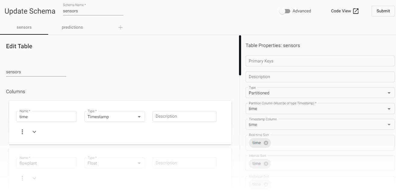
Applying the JSON will populate the schema table. -
Scroll to the bottom of the page and select Next.
- Save & Deploy the database. When the database status changes to
Active, it's ready to use.
Database warnings
Once the database is active you will see some warnings in the Issues pane of the Database Overview page, these are expected and can be ignored.

An active database, ready to use, will show a green tick next to it under the Databases menu.
2. Ingest live MQTT data
MQTT is a standard messaging protocol used in a wide variety of industries, such as automotive, manufacturing, telecommunications, oil and gas, etc.
It can be easily consumed by the kdb Insights Enterprise.
- Select Import under Discover kdb Insights Enterprise of the Overview page.
-
Select
MQTTand comeplete the properties;*are required:setting value Broker* 34.130.174.118:1883 Topic* livesensor Username* mqtt Use TLS* disabled -
Select the
JSON Decoderoption; clickNext. -
Transform data to a kdb+ database compatible format;
*are required properties.setting value Data Format* Any Click
 .
.Load
sensorsschema and the schema table created in 1. build a databaseClick
Next -
Configure the writer. Select the
manufacturingdatabase and itssensorstable. -
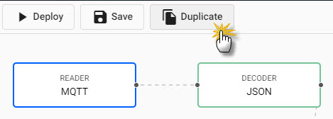
Click
 to open a view of the pipeline.
 -
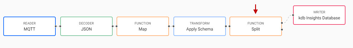
In the pipeline view, add a
FunctionMap node to the pipeline. The decode of the JSON format creates a kdb+ friendly dictionary; theFunctionMap node converts the dictionary to a kdb+ table.- Right-click the existing link between the
DecoderandTransformnode; clear to remove. - Position the
Functionnode between theDecoderandTransformnode. -
Connect the
Functionnode to theDecoderandTransformnode with a click-and-drag connect of the dot edge of the node.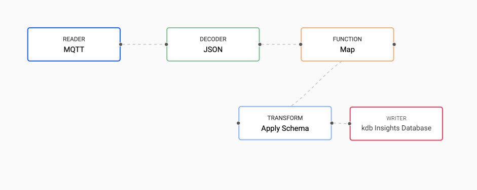
Insert theFunctionMap node between theDecoderandTransformnode. -
Select the
Functionnode and addqcode to the code editor; this transforms the kdb+ dictionary to a table:{[data] enlist data } -
Savethe pipeline -
Deploythe pipeline; complete authentication for theMQTTfeed:setting value password kxrecipe Deploying a pipeline requires an active database to receive the data; ensure the
manufacturingdatabase is deployed and active before deploying theMQTTpipeline.Check Running Pipelines of the Overview page for pipeline status; an active pipeline has
Status=RunningTrouble deploying a pipeline?
When running
Deploy, choose theTestoption to debug each node.
- Right-click the existing link between the
3. Query the data
Data queries are run in the query tab; this is accessible from the [+] of the ribbon menu, or Query under Discover kdb Insights Enterprise of the Overview page.
-
Open the Query tab.
Allow 15-20 Minutes of data generation before querying the data. Certain queries may return visuals with insufficent data if run too soon.
-
Choose
sensorsfrom theTable namedropdown. - Define the
Output variableass1. -
Define the
Start DateandEnd Time; start data is midnight of the day you deployed the pipeline to current time.
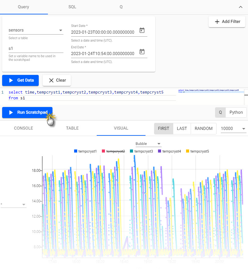
A sensors query using the filter table; start and end date use the deployment date. -
Click Get Data
- Create a visual to focus on temperature; switch the output tab to Visual
-
In the scratchpad, add the following
qcodeselect time,tempcryst1,tempcryst2,tempcryst3,tempcryst4,tempcryst5 from s1 -
Click
Run Scratchpad.In the visual, there is a cyclical pattern of temperature in the crystallizers, fluctuating between 7-20 degrees Celcius.
Get data to generate thes1output variable and run an ad hocqquery to plot sensor temperature over time in the Visual tab.Run
Get DatabeforeRun Scratchpadto create output variable.When working with scratchpad, ensure
Get Datais executed to get the output variable -
Query mass fields data in the scratchpad. Similar fluctuations occur for mass levels in the crystallizers, moving between 0-20000kg on a cycle.
select time,masscryst1,masscryst2,masscryst3,masscryst4,masscryst5 from s1
4: Define a standard compute logic
-
Continue to work in the scratchpad to set control thresholds. Use Control Chart Limits to identify predictable Upper Control (UCL) and Lower Control Limits (LCL).
Calculate a 3 sigma UCL and LCL to account for 99.7% of expected temperature fluctuations; a recorded temperature outside of this range requires investigation. In the scratchpad, paste:
// Calculating 5 new values, most notably ucl and lcl where
// ucl - upper control limit
// lcl - lower control limit
select lastTime:last time,
    lastVal: (1.0*last tempcryst3),
    countVal: count tempcryst3,
    ucl: avg tempcryst3 + (3*dev tempcryst3),
    lcl: avg tempcryst3 - (3*dev tempcryst3)
    by xbar[10;time.minute]
    from s1
Click

q/kdb+ functions explained
For more information on the code elements used in the above query:
Visualize the threshold. The change in control limits becomes more obvious in the visual appearing like the graph below after ~15-20 minutes of loading data.
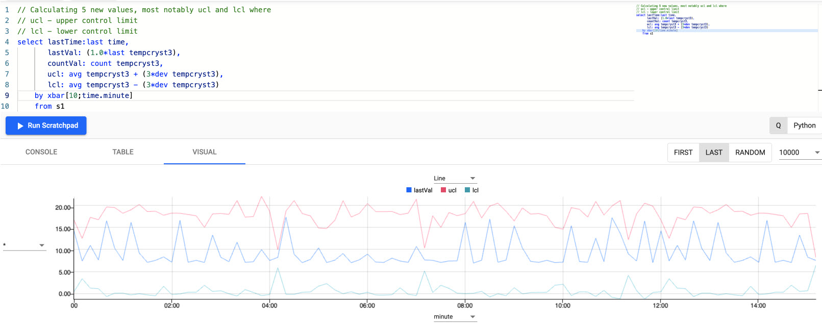
Plot of a 3 sigma upper and lower control temperature bound to account for 99.7% of expected temperature fluctuation in manufacturing process; outliers outside of this band require investigation. -
Next, aggregate temperature thresholds over two rolling time windows; a 1 minute aggregate and a second, smoother, 60 minute aggregate of sensor readings. Run in the scratchpad:
// Using asof join to join 2 tables
// with differing aggregation windows
aj[`minute;
    // table 1 aggregates every 1 minute
    select lastTime : last time,
        lastVal : last tempcryst3,
        countVal : count tempcryst3
        by xbar[1;time.minute] from s1;
    // table 2 aggregates every 60 minute
    select ucl : avg[tempcryst3] + (3*dev tempcryst3),
        lcl : avg[tempcryst3] - (3*dev tempcryst3)
        by xbar[60;time.minute] from s1]
q/kdb+ functions explained
For more information on the code elements used in the above query:
aj is a powerful timeseries join, also known as an asof join, where a time column in the first argument specifies corresponding intervals in a time column of the second argument.
This is one of two bitemporal joins available in kdb+/q.
To get an introductory lesson on bitemporal joins, view the free Academy Course on Table Joins.
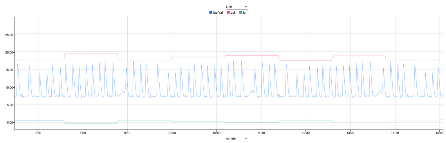
Plot of aggregate temperature thresholds for 1 minute and 60 minutes. -
Add parameters for querying; run in the scratchpad:
// table = input data table to query over
// sd = standard deviations required
// w1 = window one for sensor readings to be aggregated by
// w2 = window two for limits to be aggregated by
controlLimit:{[table;sd;w1;w2]
    aj[`minute;
    // table 1
    select lastTime : last time,
        lastVal : last tempcryst3,
        countVal : count tempcryst3
        by xbar[w1;time.minute] from table;
    // table 2
    select ucl : avg[tempcryst3] + (sd*dev tempcryst3),
        lcl : avg[tempcryst3] - (sd*dev tempcryst3)
        by xbar[w2;time.minute] from table]
 }
q/kdb+ functions explained
For more information on the code elements used in the above query:
{} known as lambda notation allows us to define functions.
It is a pair of braces (curly brackets) enclosing an optional signature (a list of up to 8 argument names) followed by a zero or more expressions separated by semicolons.
To get an introductory lesson, view the free Academy Course on Functions.
-
Define parameter values to generate thresholds; run in the scratchpad:
// By changing the parameter for w1 we can see the input sensor
// signal becoming smoother the larger we make it
controlLimit[s1;3;1;60]
controlLimit[s1;3;10;60]
controlLimit[s1;3;20;60]
4: Apply a deep neural network regression model
Apply a trained neutral network model to incoming data.

Architecture of neural network reguression model as it relates to kdb Insights Enterprise.
For the purpose of the use case, our model is pre-trained using tensorflow neural networks and xgboost. Each model prediction is then aggregated for added benefit.
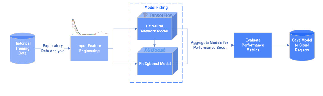
Aggregated model pre-trained using tensorflow neural networks and xgboost.
Kdb Insights Enterprise offers a range of machine learning nodes in the pipeline template to assist in model development.
-
Duplicate the pipeline created in MQTT import; give it a name
Duplicate the MQTT import pipeline from the pipeline template menu. -
In Pipeline Settings, open the Advanced accordion and paste into the Global Code editor:
import numpy as np import pykx as kx ewmaLag100 = np.nan ewmaLead100 = np.nan ewmaLag300 = np.nan ewmaLead300 = np.nan timeSince = np.nan started = False back = np.nanewmaLag100:0n; ewmaLead100:0n; ewmaLag300:0n; ewmaLead300:0n; timeSince:0n; started:0b; back:0n;Update the pipeline settings with
pythonorqcode. -
Add a Function Split node to the pipeline. Connect this node to the Transform Schema node. This split maintains the database write as one path, and adds the machine learning workflow to the second path.
Right-click a connecting link to remove it, click-and-drag on the dot to connect two nodes.
Add a Function Split node to the pipeline. -
Add a Function Map node. Cut-and-paste to the code editor using either
pythonorqcode, leave Allow Partials checked:def func(data): global timeSince, back if (data["masscryst3"][0].py()>1000)&(not np.isnan(back))&(back < 1000): timeSince = 0.0 else: timeSince = timeSince + 1.0 back = data["masscryst3"][0].py() d = data.pd() d['timePast'] = timeSince return d[['time','timePast','tempcryst4','tempcryst5']]{[data] data:-1#data; $[(first[data[`masscryst3]]>1000)&(not null back)&(back<1000); [timeSince::0; back::first[data[`masscryst3]]; tmp:update timePast:timeSince from data]; [timeSince::timeSince+1; back::first[data[`masscryst3]]; tmp:update timePast:timeSince from data] ]; select time,timePast,tempcryst4,tempcryst5 from tmp }Click

A new variable,
timePast, calculates the time interval between spikes; a spike occurs when product mass breaks above 1,000 kg - the spike threshold.Rename nodes on right-click
Right-click on a node to rename
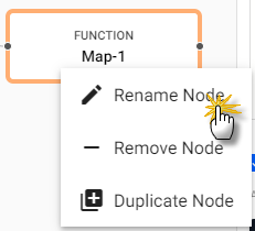
Rename a node on right-click. -
Add a second Function Map node; connect it to the spike threshold node. Cut-and-paste to the code editor in
pythonorq:def func(data): global started,ewmaLag100,ewmaLead100,ewmaLag300,ewmaLead300 a100=1/101.0 a300=1/301.0 if not started: started = True ewmaLag100 = data["tempcryst5"][0].py() ewmaLead100 = data["tempcryst4"][0].py() ewmaLag300 = data["tempcryst5"][0].py() ewmaLead300 = data["tempcryst4"][0].py() else: ewmaLag100 = a100*data["tempcryst5"][0].py() + (1-a100)*ewmaLag100 ewmaLead100 = a100*data["tempcryst4"][0].py() + (1-a100)*ewmaLead100 ewmaLag300 = a300*data["tempcryst5"][0].py() + (1-a300)*ewmaLag300 ewmaLead300 = a300*data["tempcryst4"][0].py() + (1-a300)*ewmaLead300 d = data.pd() d['ewmlead300'] = ewmaLead300 d['ewmlag300'] = ewmaLag300 d['ewmlead100'] = ewmaLead100 d['ewmlag100'] = ewmaLag100 d['model'] = kx.SymbolAtom("ANN") d = d[~(np.isnan(d.timePast))] return d{[data] a100:1%101.0; a300:1%301.0; $[not started; [ewmaLag100::first data`tempcryst5; ewmaLead100::first data`tempcryst4; ewmaLag300::first data`tempcryst5; ewmaLead300::first data`tempcryst4; started::1b]; [ewmaLag100::(a100*first[data[`tempcryst5]])+(1-a100)*ewmaLag100; ewmaLead100::(a100*first[data[`tempcryst4]])+(1-a100)*ewmaLead100; ewmaLag300::(a300*first[data[`tempcryst5]])+(1-a300)*ewmaLag300; ewmaLead300::(a300*first[data[`tempcryst4]])+(1-a300)*ewmaLead300 ]]; t:update ewmlead300:ewmaLead300,ewmlag300:ewmaLag300,ewmlead100:ewmaLead100,ewmlag100:ewmaLag100 from data; select from t where not null timePast }Click
This node calculates moving averages for temperature.
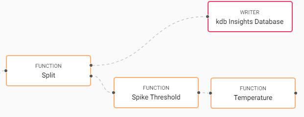
A second Function node calculates moving averages for temperature and is connected to the spike threshold node. Each function node is renamed to identify its role in the pipeline. -
Add a Machine Learning node. A large number of machine learning options are available, add the Predict Using Registry Model and connect to the temperature calculation function node.
-
Click
 to add a Feature Column Name; this is done for the variables defined in the previous function node:
setting value Feature Column Name ewmlead300 Feature Column Name ewmlag300 Feature Column Name ewmlead100 Feature Column Name ewmlag100 Feature Column Name tempcryst4 Feature Column Name tempcryst5 Feature Column Name timePast 
In the Predict Using Registry Model node, add a Feature Column Name for the variables defined in the previous function node. -
Set the remaining properties of the Predict Using Registry Model node:
setting value Prediction Column Name yhat Registry Type AWS S3 Registry Path s3://qrisk -
Click
-
-
A third Function Map node is connected to the Machine Learning node. This node adds some metadata. Copy into the
pythonorqcode editor:def func(data): d = data.pd() d['prediction'] = d['yhat'].astype(float) return d[['time','model','prediction']]{[data] select time, model:`ANN, prediction:"f"$yhat from data }Click

A third Function Map node is connected to the Machine Learning node to add some metadata. -
The final node completes the workflow with a write to the database. Connect the Writer kdb Insights database node to the metadata Function node.
setting value Database manufacturing Table predictions Write direct to HDB unchecked Deduplicate Stream checked Click
-
Savethe pipeline. In the save dialog, open Environment Variables. This step accesses the machine learning model on AWS cloud storagae.variable value AWS_ACCESS_KEY_ID AKIAZPGZITYXCEC35GF2 AWS_SECRET_ACCESS_KEY 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 AWS_REGION eu-west-1 Click
Save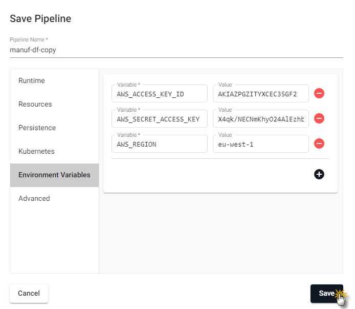
Define the Environment Variables to access the machine learning model stored on AWS. -
If still running, teardown the existing manufacturing platform and Clear Pipeline State.
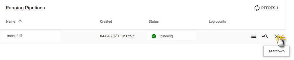
Teardown any running manufacturing pipeline before deploying the machine learning version. Check the box to Clear Pipeline State in the pop-up dialog. -
Deploy the modified pipeline with the machine learning workflow. Complete the authentication to access the
MQTTfeed:setting value Password kxrecipe Check Running Pipelines of Overview; when
Status=Runningthe prediction model has begun.When will my data be ready to Query?
It takes at least 20 minutes to calculate the
timePastvariable as two spikes are required; for more spikes in the data, shorten the frequency of spike conditions.
5. Query the Model
After sufficient time has past to generate values for timePast open the query tab; this is accessible from the [+] of the ribbon menu, or Query under Discover kdb Insights Enterprise of the Overview page.
-
Select the
Querytab. -
Define the filters:
setting value Table name predictions Output variable p1 Start date Midnight of deployment date End date 23:59 of deployment date -
Select Visual tab
-
Run

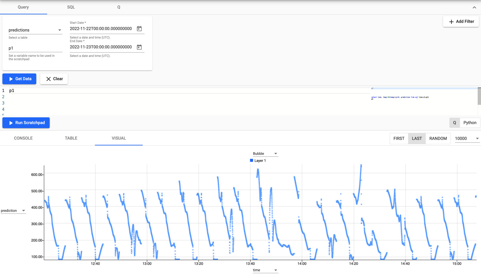
Initial predictive output from set variables. -
Compare the prediction to "real-world" data; in the scrachpad paste the code:
select time,
    temp:20*tempcryst4,      // adjust temp by a factor of 20 for visulization purposes
    prediction
    from aj[`time;s1;p1]        // joining sensors input data with predictions table on time
Click
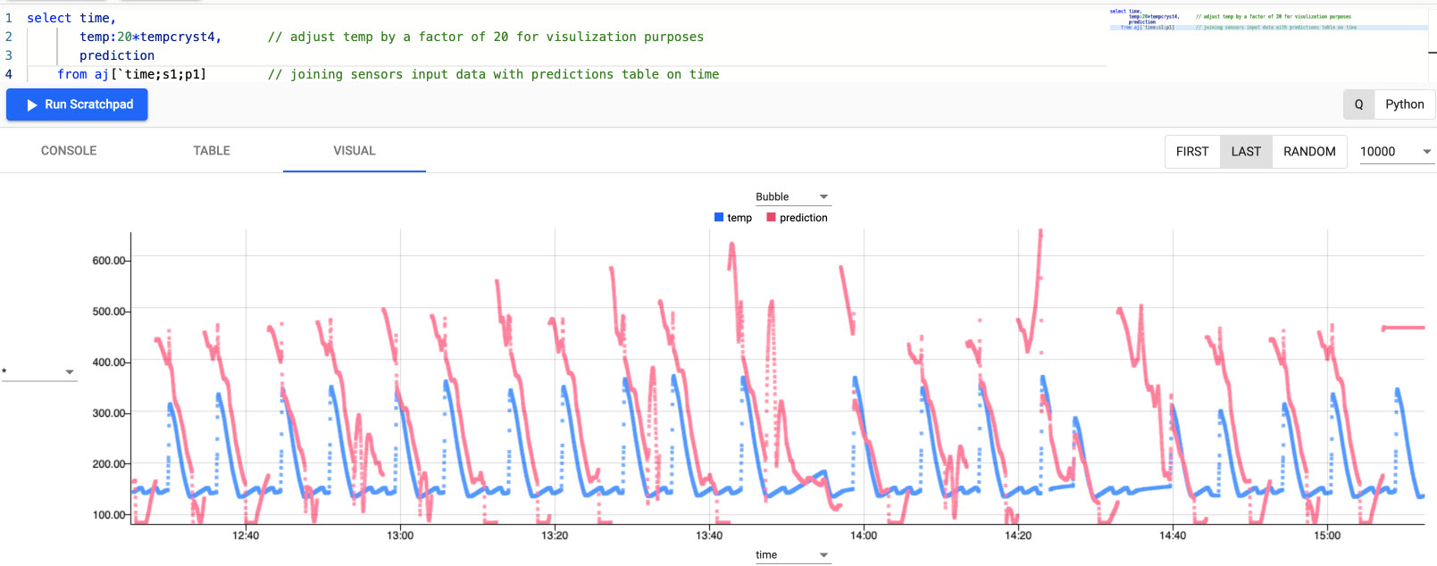
Predictive model vs real-world data.
Summary
While not perfect, the red predictive data matches relatively well to real-world data in blue. Model performance would improve with more data.
The prediction model gives the manufacturer advance notice to when a cycle begins and expected temperatures during the cycle. Such forecasting informs the manufacturer of filtration requirements.
In a typical food processing plant, levels can be adjusted relative to actual temperatures and pressures. By predicting parameters prior to filtration, the manufacturer can alter rates in advance, thus maximising yields.
This and other prediction models can save millions of dollars in lost profits, repair costs, and lost production time for employees. By embedding predictive analytics in applications, manufacturing managers can monitor the condition and performance of assets and predict failures before they happen.