Spreadsheet
The Spreadsheet provides a spreadsheet-like interface that allows you to write formulas in q and work directly with q data types like tables, dictionaries and list. It facilitates an interactive, incremental style of data analysis and allows you to capture analytical workflows and share them with colleagues. It is also useful for experimenting with and perfecting different q expressions.
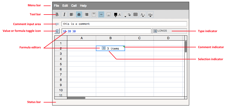
Here is a summary of the spreadsheet layout:
| location | description |
|---|---|
| Menu bar | Contains a variety of spreadsheet commands. |
| Toolbar | Contains a variety of formatting commands. |
| Comment input area | Allows you to insert a comment for each cell. When you click on the cell, the comment is displayed. To enter or edit a comment, type your comment and press the Enter key. |
| Value formula toggle | Allows you to toggle the cells between showing the q formula or the data generated by that formula. |
| Cell formula editors | Allows you to enter one or more lines of q code for the currently selected cell. To enter multiple lines, press Shift+Enter at the end of a line. |
| Cell type icon & text | Displays an icon representing the type of data in the currently selected cell. |
| Cell comment indicator | Indicates one or more cell comments. |
| Selected cell(s) indicator | When a cell is selected, the left side of the cell is coloured light blue regardless of what part of the interface is active, indicating the cell has focus. |
| Status bar | Status messages are displayed in this location. |
| Row/column sizes | Maximum number of rows is 10,000; initially set to 52. Maximum number of columns is 500; initially set to 52. |
Menu commands
File menu
| command | description |
|---|---|
| Save… | Saves the spreadsheet |
Edit menu
| command | shortcut (Windows/Linux) | shortcut (macOS) | description |
|---|---|---|---|
| Undo | Ctrl+Z | ⌘Z | Undo the last cell edit (only works in cell edit mode). |
| Redo | Ctrl+Alt+Z | ⇧⌘Z | Redo the last cell edit (only works in cell edit mode). |
| Cut cells | Ctrl+X | ⌘X | Cut selected cells |
| Copy cells | Ctrl+C | ⌘C | Copy selected cells |
| Paste cells | Ctrl+V | ⌘V | Paste selected cells and make referencing relative |
| Paste absolute | Paste selected cells but maintain current referencing | ||
| Deselect All | Ctrl+D | ⇧⌘D | Deselect all cells. |
Cell menu
| command | description |
|---|---|
| Inspect… | Opens the data inspector on the value in the selected cell. |
| History > View history | Cuts the selected range of cells. |
| Recalculate | Recalculate the selected range of cells. |
| Clear formula(s) | Clears the formulas in the selected range of cells. |
| Clear format(s) | Clears the formats in a selected range of cells. |
| Clear all formulas | Clears the formulas in the entire sheet. |
| Clear all formats | Clears the formats in the entire sheet. |
| Recalculate all | Recalculates the entire sheet. |
| Reset cell sizes | Resets the cell sizes of the entire sheet. |
| Lock/unlock selected cells | Locks or unlocks the selected range of cells. |
| Toggle selected cell formulas | Toggles the selected range of cells to always display their formulas regardless of whether the rest of the sheet is toggled to show formulas or data values. |
| Manage script regions… | Open the region pane to allow the user to create script regions, format and validation scripts. |
| Toggle all cell formulas | Toggles all cells to display either formulas or data values. Cells that have been set to “always show formula” will ignore this toggle. |
Help menu
| command | description |
|---|---|
| Open help on editor selection | Opens the q function reference in context to the current selection. |
| Keyboard reference… | Opens a dialog showing all keyboard shortcuts. |
| Q reference | Opens the q function reference guide. |
| Function reference… | Opens the function reference guide. |
| User guide | Opens user guide. |
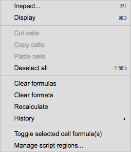
Context menu
You can invoke a context menu by right-clicking within the spreadsheet cells. The context menu contains commands from the Edit and Cell menus. Please refer to those menus for more information about the specific commands.
Create a new spreadsheet
- Select File > New… > Spreadsheet from the Explorer.
- Type a filename beginning with a period.
- Click OK.
- A new spreadsheet will appear in the Explorer.
- Double-click the spreadsheet to open it.
Selecting
Selecting a cell or cells
- Click on the cell
- To select a range of cells (e.g. B2:C5), click on a cell and drag in any direction
Selecting a row or rows
- Click on a row header
- To select multiple rows, click and drag north or south
Selecting a column or columns
- Click on a column header
- To select multiple columns, click and drag left or right
Editing content
Entering q formulas in a cell
There are multiple ways of entering formulas into a cell.
- Select a cell in the spreadsheet or double-click the cell or just start typing in a cell.
- A cell editor will appear in the cell location.
- As you type, both the cell editor and formula bar at the top of the display will update accordingly.
- Unlike Excel, you do not enter an equal sign at the start of a formula.
- Press Enter or click on a different cell.
- The q formula will be added to the cell and the resulting data value will appear in the cell.
- Single-clicking on a cell will show the formula in the formula bar.
Entering an embedded comment in a cell
- Select a cell.
- Enter two forward slashes followed by some text.
- Press Shift+Enter to move to the next line in the cell.
- Enter a q formula into the cell. Note that the embedded comment is not displayed as a cell value, however, it can still be seen in the formula editor at the top of the window. In other words, to view an embedded comment you must first select the cell and then look at the formula editor.
- Note that comments embedded in formulas are different from cell comments, which appear at the top of the window in the comment area. If there are cell comments this is indicated by a green triangle icon in the upper right corner of the cell. To create a cell comment, type in the cell comment area.
Understanding cell types and type icons
When you click on a cell, you will see the type icon and text are updated in the top right corner of the spreadsheet. The table below summarizes the data types and their icons.

Here is a summary of the icons:
| icon | type | icon | type |
|---|---|---|---|
 |
binary |  |
List with text name of the type (e.g. INTS) |
 |
boolean |  |
Long |
 |
byte |  |
Minute |
 |
character |  |
Month |
 |
composition |  |
Projection |
|
date |  |
Real |
|
dateTime | |
Second |
 |
dictionary |  |
Short |
 |
dynamicLoad |  |
Symbol |
| empty |  |
Table | |
|
enumerations |  |
Ternary |
 |
float | |
Time |
 |
general | |
TimeSpan |
 |
integer | |
TimeStamp |
 |
lambda |  |
Unary |
 |
error |
Referencing a q cell from another cell
From any cell, you may refer to any other cell using standard Excel-like column-row notation. You may enter uppercase or lowercase cell references (e.g. A1).
In the example, below the value B1[A1] has been entered into cell C1.
Cell A1 contains the integer 23.
Cell B1 contains a lambda function that will multiply any value it is given by 2.
Cell C1 calls the B1 function with cell A1 as the argument.
You can see the formula in the formula bar at the top of the page and the output value in the C1 cell.
Double-clicking the C1 cell will also let you edit the cell in place.

Referencing cell ranges
You can specify a range of rows, a range of columns, or a range of rows and columns in your commands by specifying the starting and ending cell within a set of brackets as shown below.
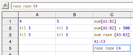
In cell C1, the user enters the q sum function with a range of cells starting at A1 and ending at B1.
The returned result is the sum of the two cells.
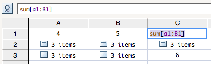
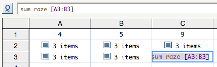
However, you can also sum cells that contain lists of items. In this example, A2 and B2 contain lists. In this case, the user sums the cells. C1 returns a list that contains the sum of each index in the list.
If you want conventional spreadsheet behavior, you would need to
flatten the list of columns using raze, then sum the items to obtain
the single sum value.
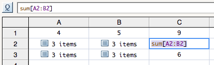
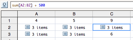
Q programming techniques allow you to perform powerful operations against lists, tables, and dictionaries. In this example, in C2 we perform the same operation as above and then add 500 to each value in the resulting list.
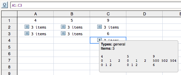
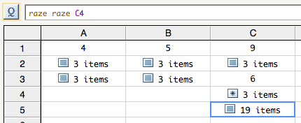
It is important to understand that the definition of a range preserves
the row-column data so that the data can be operated on using q
programming techniques.
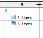
As shown in the example below, if we enter the
range [A1:C3] in cell C4, the result is three 3-item lists (i.e.
a 3×3 array).
Ranges
Ranges are always interpreted as upper-left to bottom-right regardless of how they are enumerated, e.g., A1:A5 and A5:A1 are always interpreted as the same range.
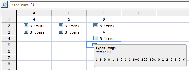
However, if we want a simple list to be returned, then we must use the raze function to deconstruct the array.
Toggling the function or data view of the spreadsheet cells
You can look at either a data view or a function view of the spreadsheet by toggling between the two views. To toggle between the views, click the icon circled below. Depending on the view it will display either the Q icon or the Fx icon.
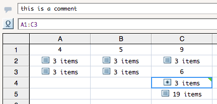
Alternatively, you can have some cells permanently display their formulas. In this example, cell C5 was toggled to always show its formula using the Cell > Toggle always show formula command. Notice that the Q data value icon is showing but the formula in C5 is displayed regardless. You will also notice a thin vertical highlight line at the front of the C5 cell. This line indicates that the cell is toggled to show its formula.

Updating a cell
You can update cells in the spreadsheet.
- Select a cell.
- Pick History > View history… from the Cell or context menu.
- The History Dialog will appear.
-
Select the version you wish to update to from the dialog.
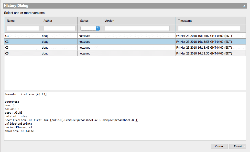
-
Click the Revert button.
The cell will update with the selected content.
Entering a comment marker
- Select a cell
- Type a comment into the text line at the top of the display as shown below.
- Click on another cell.
The comment indicator icon will appear in the cell.
Editing a comment marker
- Select a cell.
- Change the text in the comment area.
- Click on another cell.
Deleting a comment marker
- Select a cell.
- Remove the text from the comment area.
- Click on another cell.
The comment icon will disappear.
Resizing
Resizing a cell manually
You can resize the height or width of a cell or range of cells.
- Select the row range or column range as described previously.
-
Move the cursor to the end of the range until the resize cursor appears:
-
Drag the row or rows vertically or column or columns horizontally. A pale blue drag box appears as you drag.
-
Release the mouse and the cell range will resize. In the case of a range of cells, the width of the selection area is divided by the number of columns or rows selected. For example, if you have selected three columns and you resize the range to 75 pixels, each column will be 25 pixels wide. There are minimum settings for columns (35 pixels) and rows (21 pixels).

Resizing a cell by numeric value
-
Select a range of rows or columns.
-
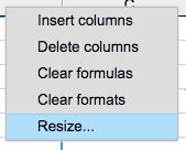
Right-click on the row or column header to see the context menu.
-
Pick Resize… from the context menu.
-
Type a data value into the row or column resize dialog and click OK.
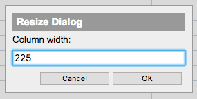
The row or column will resize.
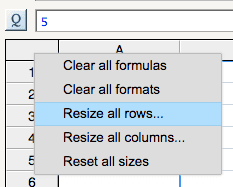
Resizing all rows or columns
In the top-left corner of the spreadsheet pick Resize all rows… from the context menu.
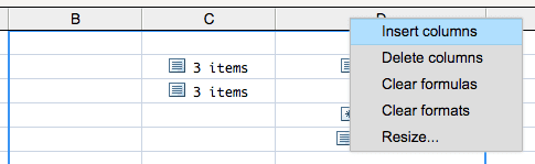
Inserting a row or column
- Select the number of rows or columns you wish to insert. For example, if you wish to insert 3 columns after column A, select columns B, C and D.
- Right-click on a row or column header.
-
Pick Insert rows or Insert columns from the context menu.
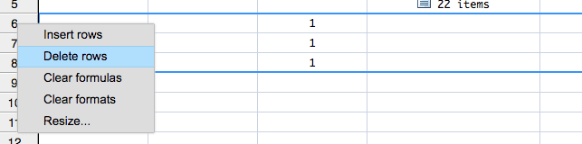
Deleting a row or column of cells
- Select the number of rows or columns you wish to delete. For example, if you wish to delete rows 6, 7, and 8, select them.
- Right-click on a row or column header.
-
Pick Delete rows or Delete columns from the context menu.
Clearing content
Clearing formulas from a cell or cell range
- Select a cell or cell range
- Pick Clear formula(s) from the Edit or context menu
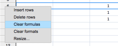
Clearing formulas from a row
- Select a row header or range of row headers.
- Right-click on the row header.
-
Pick Clear formulas from the context menu.
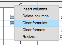
Clearing formulas from a column
- Select a column header or range of column headers.
- Right-click on the column header.
-
Pick Clear formulas from the context menu.
Clearing a cell or a range of cells
- Select the cell or cell range you wish to delete.
- Press the Delete key or pick Clear formula(s) from the Cell or context menu.
Formatting cells
Cells can be formatted using the toolbar at the top of the spreadsheet. Select the cell or range of cells you wish to format and click the appropriate icons.
| icon | description |
|---|---|
| Bold the selected cell range | |
| Italicize the selected cell range | |
| Left align the selected cell range | |
| Centre align the selected cell range | |
| Right align the selected cell range | |
| Top align the selected cell range | |
| Middle align the selected cell range | |
| Bottom align the selected cell range | |
| Colour the foreground text | |
| Colour the background cell | |
| Turn the grid on or off | |
| Change the type size | |
| Change the type font family |
Excel differences
Here are some differences from Excel spreadsheets.
-
Use of equal sign is unnecessary. You do not need to enter an equal sign (
=) in the formula bar. The formula bar takes data values or any q expression and evaluates them. -
Individual cell insertion is not supported. You can only insert full rows or columns.
-
Decimal formatting is not supported. You can set decimal formatting via q commands only.
-
Ranges work differently. If you specify a range
[A1:C1], an array of the values contained in those cells is returned, and operations may be performed on the array. This will return a list of lists representing a 3×2 array. This aligns nicely with q semantics and allows you to perform a wide range of computations against the contents of tables, lists and dictionaries. However, if you want more Excel-like behavior, you need to use therazefunction to deconstruct the range array. In this case, we wouldrazecell C3 and thensumthe values to get the Excel-like behavior. -
Ranges include blank cells in the computation and treat them as zero. In the example below, we have three cells B2=3, C2=Empty, and D2=5. If we were to evaluate this cell range looking for an average (e.g.
avg B2:D2), it would return 2.666667 instead of 4 because the empty cell is treated as zero (e.g.3+0+5divided by 3)
Spreadsheet usages
The Spreadsheet can be used in two ways:
- As a spreadsheet with default spreadsheet behavior
- As a spreadsheet with a custom user interface containing format and validation scripts
Each way is described below in further detail.
Spreadsheet with default spreadsheet behavior
To make the spreadsheet usage more concrete, let’s convert this three-line q script from a text editor view into a spreadsheet view.
In the example, n is assigned a value of 1000, stocks are assigned several values, and then these values are used to randomly populate a table that would emulate some trades on the New York Stock Exchange.
n:1000;
stocks:`ibm`amazon`apple`intel`nortel`att`siemens`alcatel`lucent`hp;
nyse:([]stock:n?stocks;price:n?100.0;amount:100_10+n?20;time:n?24:00:00.000)
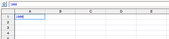
To convert this script, the user types 1000 into A1 without the variable name.
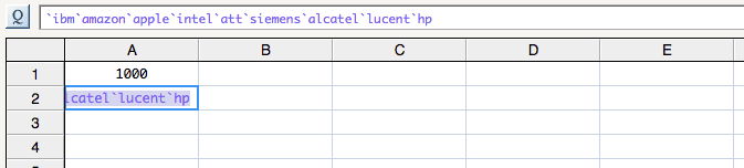
The user then types
`ibm`amazon`apple`intel`nortel`att`siemens`alcatel`lucent`hp
into A2.
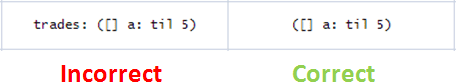
When the user presses Enter, the cell updates with the values and the list icon, symbol icon and word `symbol appear to let the user know that they have created a list of symbols.
Notice that they no longer use the variable stock.
The user then types
([]stock:A1?A2;price:A1?100.0;amount:100_10+A1?20;time:A1?24:00:00.000)
into A3. When the user presses Enter, the cell updates with the values and the table icon is displayed to show the user that a table resides in the cell.
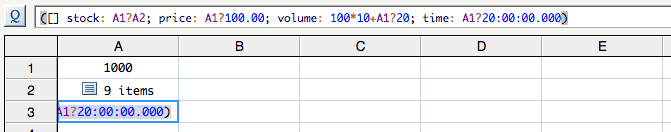
Hovering the cursor over the table icon, gets a summary of the data in the table.
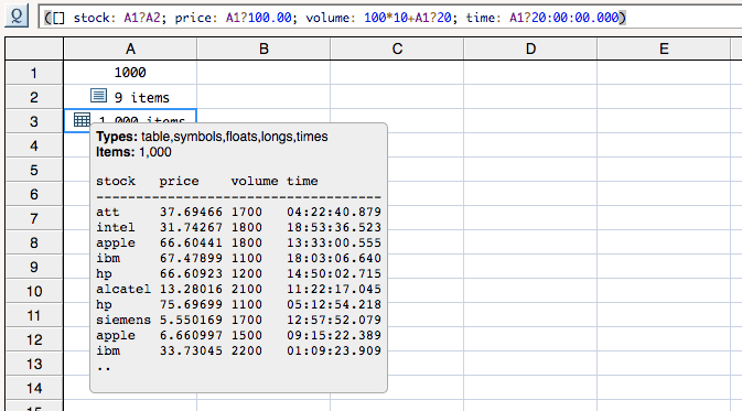
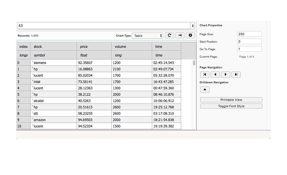
If the user inspects cell A3, the table is displayed in the Visual Inspector.
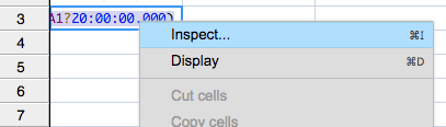
By default, the Visual Inspector displays a textual table. Here we can see that it contains 1000 stock records.
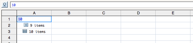
If the user modifies the value in A1 to 10, the cells are recalculated.
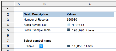
Spreadsheet with customized user interface
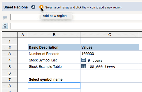
In the example below, a developer has created a custom user interface with a dropdown combo box (B9) that will allow novice users to enter data into the spreadsheet easily. The data can then be used by the spreadsheet or another function to perform data analysis. In order to create the customized interface, the developer added cell regions to the spreadsheet. Then she added format and validation scripts to those regions. Format scripts change the appearance or format of a cell. Validation scripts check or validate the values entered into a cell. JavaScript is used as the scripting language for creating format and validation scripts.
Format scripts
Format scripts are intended for modifying the output display of a cell. As such, script commands that update or modify cell formulas should not be used in a format script as they will cause cycle errors in your spreadsheets.
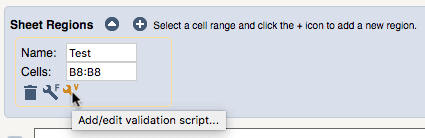
In the example below, the cell region pane has been opened. We can see that a cell region has been defined for B8. This cell region contains a format script to display the combo box.
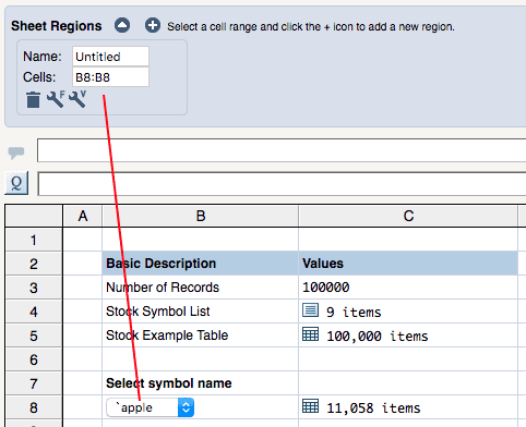
The format script below displays a combo box in every cell that is within the region. In this case, the region is defined as B8:B8. That means the script will display only one combo box. The script gets the contents of the cell object for C4 and creates an array. It then modifies each value and uses them to fill the combo box display values.
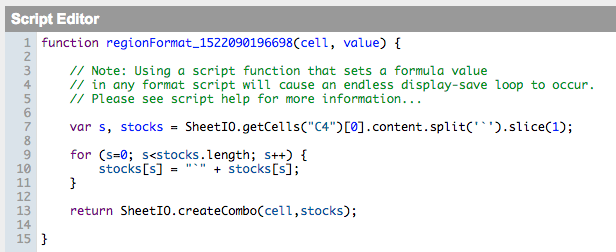
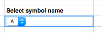
Once the format script is saved, the user can select from the combo box.
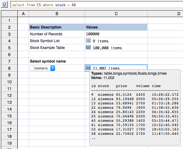
In this case, cell C8 contains a query that relies on cell B8.
When the combo box value changes (e.g. `siemens), the query in cell C8 is run against the table in cell C5 and the appropriate results are returned.
In this example 11,002 records match the stock.
Here are the steps to create this kind of script:
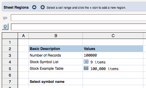
-
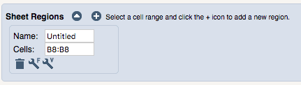
Open the script region pane. Pick Manage script regions… from the Cell menu and the cell region pane will appear. (Initially, it will be empty, as shown.)
-
Add a cell region. With the region pane open, select B2 and click the plus icon to add a cell region.
A cell region is added in the region pane.
-
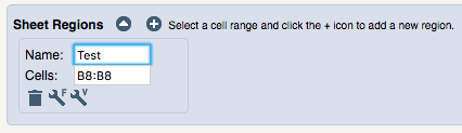
Name a cell region. With the region pane open, click on the name field edit the name and press Enter. The name changes.
-
Change the bounds of a cell region. With the region pane open, click on the cells field; edit the cell range and press Enter. The cell range updates in the spreadsheet.

-
Delete a cell region. With the region pane open, click on the garbage can to delete a cell region. The region is removed from the spreadsheet.
-
Save a cell region. Regions are saved any time there is a change. However, you can also explicitly save the region: click the disk icon.
-
Add a format script to a cell region. With the region pane open, click on the F wrench icon.
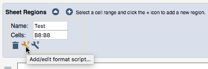
A script editor dialog will appear.
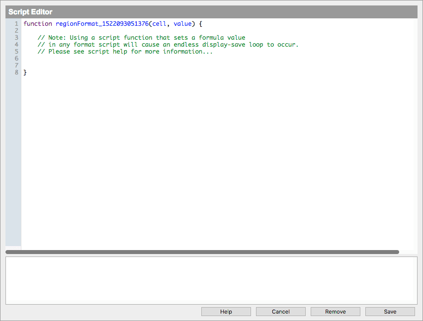
A format script must return a valid HTML string. In this example, all cells in the region would be populated with a combo box containing three values (e.g.
`A,`B,`C). However, no value has actually been added to the cell’s formula at this point. To add a value to the cell, the user would have to make a selection.Helper functions are available to help you write scripts. To learn more about the helper functions, click the Help button in the script dialog.
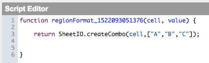
Click the Save button at the bottom of the dialog to save the script. The display will update showing a combo box in the appropriate cell location.
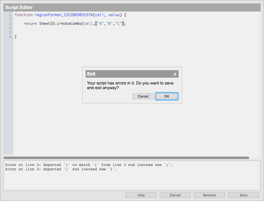
Sometimes after clicking the Save button, the script is run through jsLint to help you improve your code quality. In this example, the closing parenthesis has been omitted to demonstrate the linter. However, you can always save your script even if it contains jsLint errors.
-
Add a validation script to a cell region. With the region pane open, click on the V wrench icon.
A script editor dialog will appear.
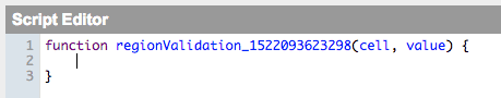
A validation script must return either true or false. Validation scripts are executed just prior to saving a cell. If the script returns
true, the formula entered will be saved to the server. If the script returnsfalse, the formula is not saved. In this example, the validation script looks at the value of the cell. If the value is contained in the values collection, then the result flag is set totrue. Otherwise the result flag remainsfalse.Helper functions are available to help you write scripts. To learn more about the helper functions, click the Help button in the script dialog.

Click the Save button at the bottom of the dialog to save the script. After clicking the Save button, the script is run through jsLint to help you improve your code quality. However, you can always save your script even if it has jsLint errors.
Adding graphs
Graphs can be added to a spreadsheet by clicking the Add graph icon in the toolbar:

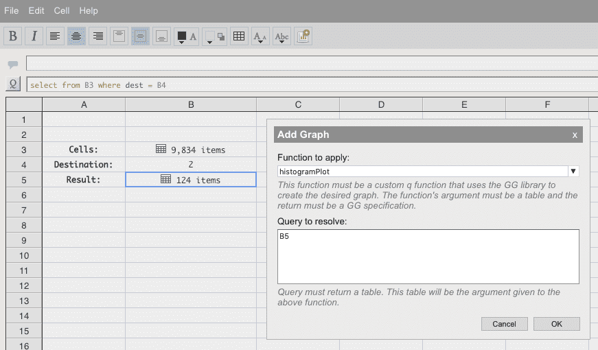
When clicked, a dialog will appear where a function can be chosen from the workspace, and a query can be entered.
- The function must take a single table as an argument, and return a Grammar of Graphics specification. For example, the
B3table has adurationcolumn below, so a histogram could be constructed by defining the following workspace function:
histogramPlot: { .qp.histogram[x; `duration; ::] }
- The query must result in a table that will be passed to the plot function above. Any spreadsheet expression can be entered here, either writing q, cell references, or both, as explained in the above sections.
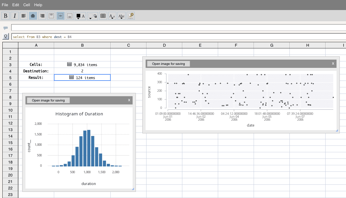
When OK is pressed on the dialog, the plot will appear within the sheet and can be resized and positioned as desired. The plot will update automatically when cells are updated just like other cells. The plot will also save with the sheet and will be present upon closing and reopening the sheet.
Known spreadsheet issues
-
Strings must be quoted. For example, if you want to enter
Header, you must enter"Header". However, spreadsheet labels can be entered into a cell as a comment by using the forward slash, e.g./this is a comment. -
It is possible to reference cells that are out of range. The maximum number of rows in a spreadsheet is 10000. The maximum number of columns is 1352. If you reference a column or row outside this range, you will get an undefined variable.
-
Variables should not be used in cells. Use cell referencing (e.g. A1) only. The spreadsheet cannot resolve variables that are not declared.
-
Certain q commands do not work because they are confused with cell names. For example,
md5andwj1resolve to 0 -
Typing whitespace (e.g. a space) or comments (e.g.
/my comment) into a cell resolves the cell to 0 in order to allow computation over column ranges. -
Zooming in and out will cause cell misalignments and/or JavaScript type errors as it is not supported.
-
Error messages in sheet applications are not reported to the user interface. If you define an error message in your custom application, the message is currently not reported in the user interface. Instead you will get the generic message for that particular API call.