Finance - Develop Trading Strategies
This page provides an example of how to use kdb Insights Enterprise to work with both live and historical data.
kdb Insights Enterprise can be used to stream live data along with historical tick data to develop interactive analytics; powering faster, and better in-the-moment decision-making. This provides the following benefits:
- Streaming live tick data alongside historical data provides the big picture view of the market which enables you to maximize opportunities.
- Real-time data enables you to react to market events as they happen to increase market share through efficient execution.
- Aggregating multiple liquidity sources provides for a better understanding of market depth and trading opportunities.
Financial dataset
The example in this page provides a real-time price feed alongside historical trade data. The real-time price feed calculates two moving averages. A cross between these two moving averages establishes a position (or trade exit) in the market. The following sections guide you through the steps to:
- Build a database
- Build the pipeline to ingest live data
- Build the pipeline to Ingest historical data
- Query the data
- Create powerful analytics
- Visualize the data
Build a database
-
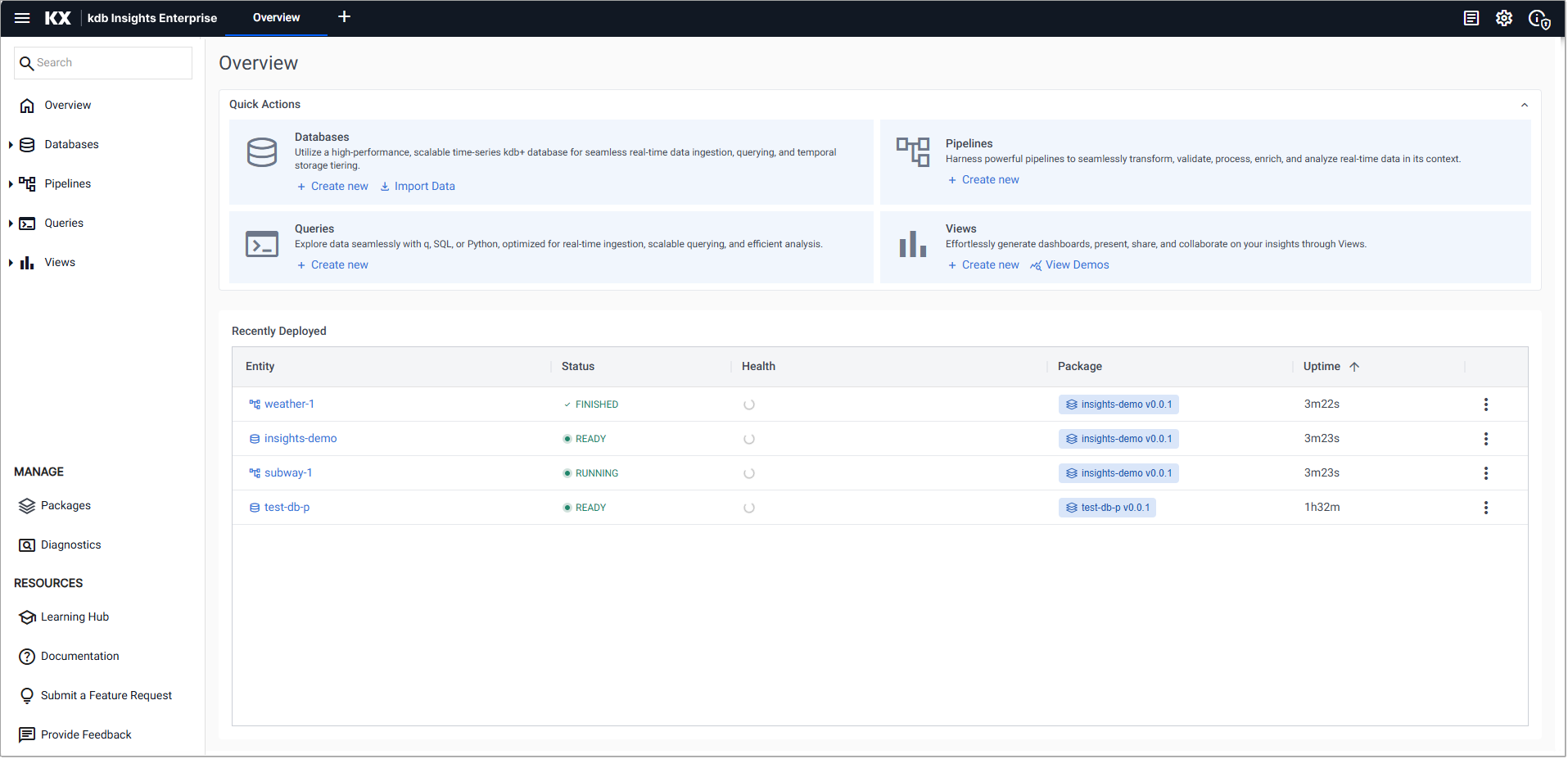
Click Create new under Databases in the Quick Actions panel, on the Overview page.
-
In the Create Database dialog and set the following:
Setting Value Database Name equities Select a Package Create new package Package Name equities -
Click Create.
-
On the Schema Settings tab click Code View to open the Schema Code View. You can use this to add large schema tables, in JSON format.
-
Replace the existing code with the following JSON to setup the
equitiesschema.equities schema
Paste the JSON code into the code editor:
[ { "columns": [ { "attrDisk": "sorted", "attrOrd": "sorted", "description": "KXI Package Schema Column", "name": "timestamp", "type": "timestamp", "compound": false, "attrMem": "", "foreign": "" }, { "description": "KXI Package Schema Column", "name": "price", "type": "float", "compound": false, "attrMem": "", "attrOrd": "", "attrDisk": "", "foreign": "" }, { "description": "KXI Package Schema Column", "name": "volume", "type": "int", "compound": false, "attrMem": "", "attrOrd": "", "attrDisk": "", "foreign": "" } ], "description": "KXI Package Schema", "name": "trade", "primaryKeys": [], "prtnCol": "timestamp", "sortColsDisk": [ "timestamp" ], "sortColsMem": [], "sortColsOrd": [ "timestamp" ], "type": "partitioned" }, { "columns": [ { "description": "KXI Package Schema Column", "name": "Date", "type": "date", "compound": false, "attrMem": "", "attrOrd": "", "attrDisk": "", "foreign": "" }, { "attrDisk": "sorted", "attrOrd": "sorted", "description": "KXI Package Schema Column", "name": "Time", "type": "timestamp", "compound": false, "attrMem": "", "foreign": "" }, { "description": "KXI Package Schema Column", "name": "Open", "type": "float", "compound": false, "attrMem": "", "attrOrd": "", "attrDisk": "", "foreign": "" }, { "description": "KXI Package Schema Column", "name": "High", "type": "float", "compound": false, "attrMem": "", "attrOrd": "", "attrDisk": "", "foreign": "" }, { "description": "KXI Package Schema Column", "name": "Low", "type": "float", "compound": false, "attrMem": "", "attrOrd": "", "attrDisk": "", "foreign": "" }, { "description": "KXI Package Schema Column", "name": "Close", "type": "float", "compound": false, "attrMem": "", "attrOrd": "", "attrDisk": "", "foreign": "" }, { "description": "KXI Package Schema Column", "name": "AdjClose", "type": "float", "compound": false, "attrMem": "", "attrOrd": "", "attrDisk": "", "foreign": "" }, { "description": "KXI Package Schema Column", "name": "Volume", "type": "long", "compound": false, "attrMem": "", "attrOrd": "", "attrDisk": "", "foreign": "" }, { "description": "KXI Package Schema Column", "name": "AssetCode", "type": "symbol", "compound": false, "attrMem": "", "attrOrd": "", "attrDisk": "", "foreign": "" } ], "description": "KXI Package Schema", "name": "close", "primaryKeys": [], "prtnCol": "Time", "sortColsDisk": [ "Time" ], "sortColsMem": [], "sortColsOrd": [ "Time" ], "type": "partitioned" }, { "columns": [ { "attrDisk": "sorted", "attrOrd": "sorted", "description": "KXI Package Schema Column", "name": "timestamp", "type": "timestamp", "compound": false, "attrMem": "", "foreign": "" }, { "description": "KXI Package Schema Column", "name": "vwap", "type": "float", "compound": false, "attrMem": "", "attrOrd": "", "attrDisk": "", "foreign": "" }, { "description": "KXI Package Schema Column", "name": "twap", "type": "float", "compound": false, "attrMem": "", "attrOrd": "", "attrDisk": "", "foreign": "" }, { "description": "KXI Package Schema Column", "name": "open", "type": "float", "compound": false, "attrMem": "", "attrOrd": "", "attrDisk": "", "foreign": "" }, { "description": "KXI Package Schema Column", "name": "high", "type": "float", "compound": false, "attrMem": "", "attrOrd": "", "attrDisk": "", "foreign": "" }, { "description": "KXI Package Schema Column", "name": "low", "type": "float", "compound": false, "attrMem": "", "attrOrd": "", "attrDisk": "", "foreign": "" }, { "description": "KXI Package Schema Column", "name": "close", "type": "float", "compound": false, "attrMem": "", "attrOrd": "", "attrDisk": "", "foreign": "" } ], "description": "KXI Package Schema", "name": "analytics", "primaryKeys": [], "prtnCol": "timestamp", "sortColsDisk": [ "timestamp" ], "sortColsMem": [], "sortColsOrd": [ "timestamp" ], "type": "partitioned" } ] -
Click Apply.
-
Click Save.
Ingest live data
The live data feed uses Apache Kafka. Apache Kafka is an event streaming platform whose data is easily consumed and published by kdb Insights Enterprise.
-
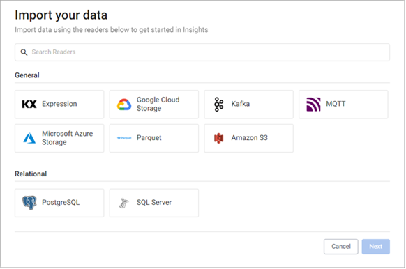
On the Overview page, choose Import Data under Databases:
-
In the Import your data screen select Kafka.
-
In the Configure Kafka screen set the following:
Setting Value Broker* kafka.insights-data.kx.com:443 Topic* spx Keep the default values for the following settings.
Setting Value Offset* End Use TLS Unchecked Use Schema Registry Unchecked -
Expand the Advanced parameters section and tick Advanced Broker Options.
-
Click +, under Add an Advanced Configuration, to add the following key value-pairs:
Key Value sasl.username demo sasl.password demo sasl.mechanism SCRAM-SHA-512 security.protocol SASL_SSL -
Click Next.
-
In the Select a decoder screen click JSON.
- In the Configure JSON screen click Next, leaving Decode each unchecked.
-
In the Configure Schema screen:
-
Leave the value of Data Format set to Any
-
Click the Load Schema icon
 and select the following values:
Setting Value Database equities(equities) Table trade
-
-
Click Load, and then click Next.
-
In the Configure Writer screen define the following settings:
Setting Value Database equities (equities) Table trade Keep the default values for the following settings.
Setting Value Write Direct to HDB Unchecked Deduplicate Stream Checked Set Timeout Value Unchecked -
Click Create Pipeline to display the Create Pipeline dialog, and select the following values:
Setting Value Pipeline Name equities-1 Select a Package equities -
Click Create.
-
In the pipeline template, click and drag the Map Function node into the pipeline template workspace.
- Right-click on the join between the Decoder and Transform nodes and click Delete Edge.
-
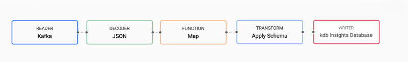
Insert the Map function between the Decoder and Transform nodes by dragging-and-connecting the edge points of the Decoder node to the Map node, and from the Map node to the Transform node, as shown below.
-
Click on the Map function node. In the Q tab of the Configure Map Node panel replace the code with the following.
{[data]
    enlist data
}
-
Click Apply to save the details to the node.
-
Click Save.
Ingest historical data
Historic data is kept on object storage, on Amazon S3.
-
On the Overview page, choose Import Data under Databases in the Quick Actions panel.
-
In the Import your data screen select Amazon S3.
-
In the Configure Amazon S3 screen:
-
Complete the properties:
Setting Value S3 URI* s3://kxs-prd-cxt-twg-roinsightsdemo/close_spx.csv Region* eu-west-1 Tenant kxinsights Keep the default values for the following settings.
Setting Value File Mode* Binary Offset* 0 Chunking* Auto Chunk Size* 1MB Use Watching Unchecked Use Authentication Unchecked -
Click Next
-
-
In the Select a decoder screen click CSV and keep the default settings.
- In the Configure CSV screen keep all the default values and click Next.
-
In the Configure Schema screen:
- Leave Data Format unchanged as Any
- Click the Load Schema icon , and select the following values:
Setting Value Database equities(equities) Table close - Click Load to apply the schema, and click Next.
-
In the Configure Writer screen:
- Define the following settings:
Setting Value Database equities (equities) Table close Keep the default values for the following settings.
Setting Value Write Direct to HDB Unchecked Deduplicate Stream Checked Set Timeout Value Unchecked - Click Open Pipeline.
-
In the Create Pipeline screen select the following values:
Setting Value Pipeline Name close-1 Select a Package equities - Click Create
-
Click Save.
-
Click on Packages, in the left-hand menu to open the Packages index.
-
Click on the three dots to the right of the equities package and click Deploy.
The Deploy Package dialog open. Click Deploy.
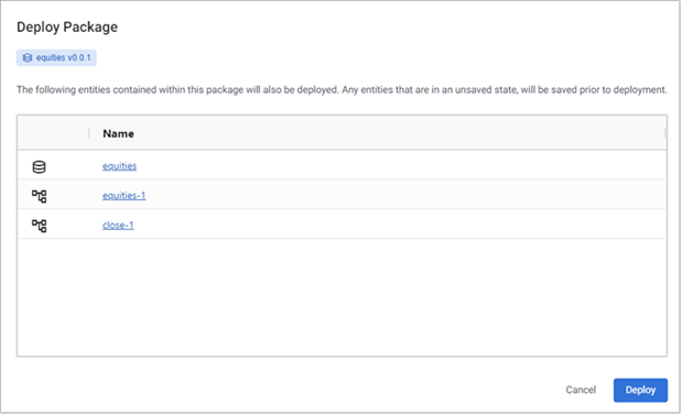
Deploying the package, deploys the database and associated pipelines. These read the data from its sources, transform it to a kdb+ compatible format, and write it to the database.
When the Status of the package updates to RUNNING the package has been deployed.
-
To verify the status of all deployed entities, click on Overview to view the Recently Deployed table, and confirm the status of the following.
Entity Status equities Ready equities-1 Running close-1 Finished
Query the data
-
Click + on the ribbon menu and click Query.
-
Click the SQL tab, on the Query & Load Data panel, and enter the following command to retrieve a count of streaming events in the trade table:
SELECT COUNT(*) FROM trade -
Define the Output Variable as t.
-
Click Run Query. The results are displayed in the lower part of the Query screen, as shown below.
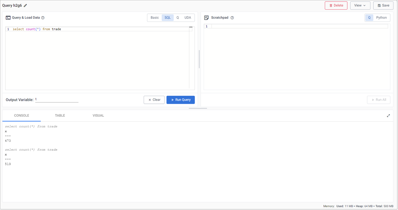
Re-run the query to get an updated value.
-
Right-click in the Console and click Clear to clear the results.
-
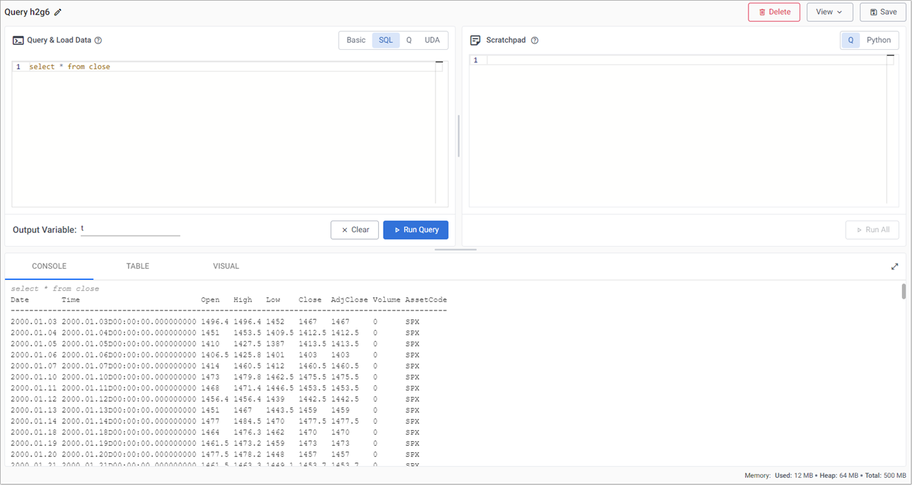
In the SQL tab, replace the existing code with:
SELECT * FROM close -
Define the Output Variable as t.
-
Click Run Query. The results are displayed in the Console as illustrated in the example below which shows end-of-day S&P historic prices.
Create powerful analytics
Using the data, a trade signal is created to generate a position in the market (S&P).
-
Replace the query, in the SQL tab, with the following:
SELECT * FROM trade -
Set the Output Variable to t.
-
Click Run Query.
-
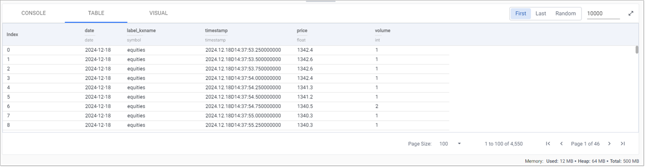
In the output section, toggle between Console, Table or Visual for different views of the data. For example, a chart of prices over time.
- Click Run Query after changing tabs. The following screenshot shows an SQL query against streaming trade data, viewed in the Table tab.
Long and short position simple moving averages
This strategy calculates two simple moving averages, a fast short time moving average, and a slow long time period moving average.
When the fast line crosses above the slow line, we get a buy trade signal, with a sell signal on the reverse cross.
This strategy is also an always-in-the-market signal, so when a signal occurs, it not only exits the previous trade, but opens a new trade in the other direction; going long (buy low - sell high) or short (sell high - buy back low) when the fast line crosses above or below the slow line.
-
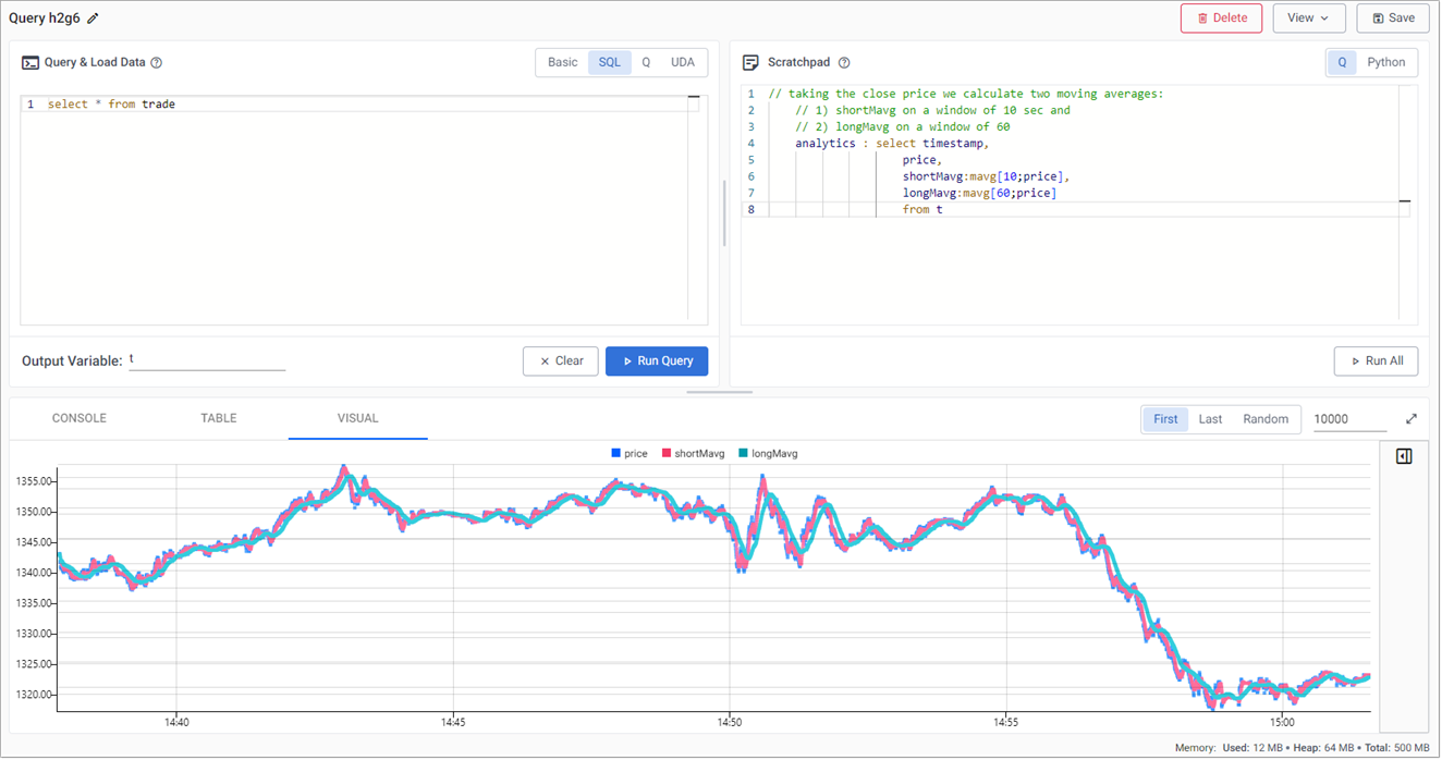
In the q tab of the Scratchpad panel, in the query window, enter the following code to create a variable analytics to calculate the fast and slow moving average.
// taking the close price we calculate two moving averages: // 1) shortMavg on a window of 10 sec and // 2) longMavg on a window of 60 analytics : select timestamp, price, shortMavg:mavg[10;price], longMavg:mavg[60;price] from t -
Click Run All.
This strategy uses a 10-period moving average for the fast signal, and a 60-period moving average for the slow signal. Streamed updates for the moving average calculations are added to the chart, as illustrated below.
Trade position
The crossover of the two fast and slow moving averages creates trades. These can be tracked with a new variable called positions.
-
In the scratchpad, append the following:
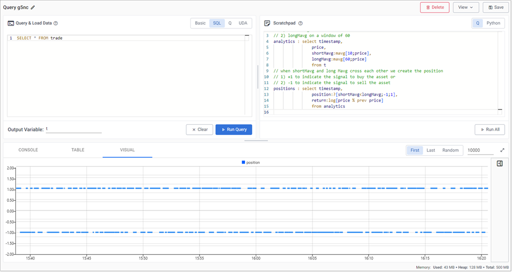
// when shortMavg and long Mavg cross each other we create the position // 1) +1 to indicate the signal to buy the asset or // 2) -1 to indicate the signal to sell the asset positions : select timestamp, position:?[shortMavg<longMavg;-1;1], return:log[price % prev price] from analytics -
Click Run All. A position analytic to track crossovers between the fast and slow moving averages is displayed in the query visual chart, as shown in the following screenshot.
q/kdb+ functions explained
If any of the above code is new to you don't worry, we have detailed the q functions used above:
| Function | Description |
|---|---|
| ?[x;y;z] | When x is true return y, otherwise return z |
| x<y | Returns true when x is less than y, otherwise return false |
| log | To return the natural logarithm |
| x%y | Divides x by y |
Active versus passive strategy
The current, active strategy is compared to a passive strategy; that is a strategy tracking a major index, like the S&P 500 or a basket of stocks, such as an ETF. We want to know if our strategy performs better.
Use this link to learn more about active and passive strategies
-
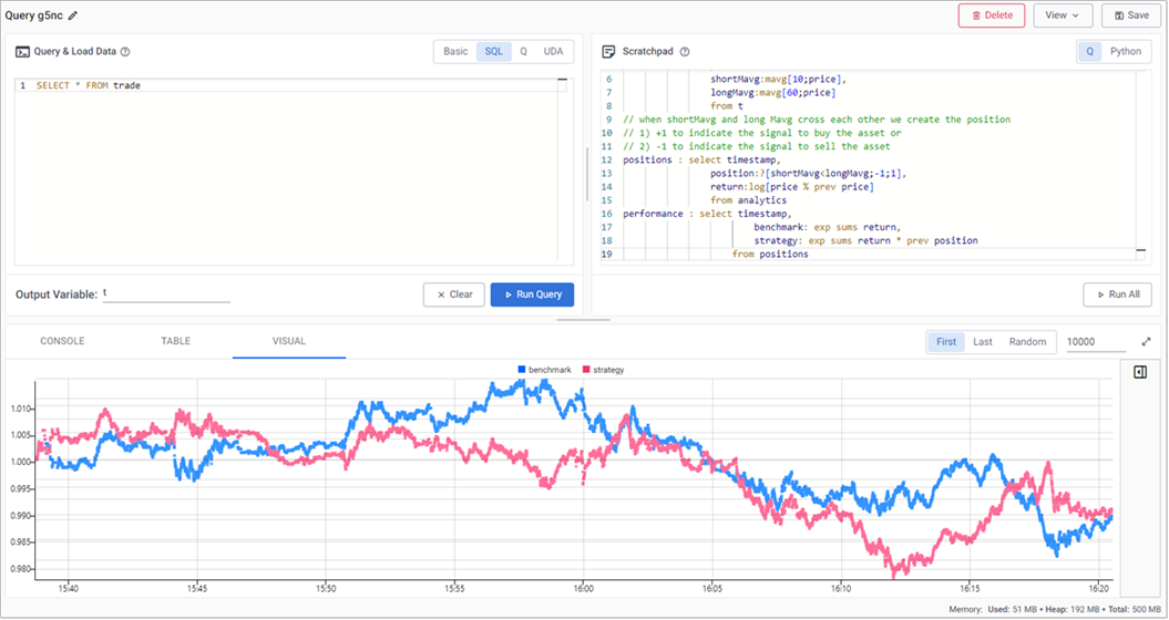
In the Scratchpad, append the following code, to create a new variable called performance which generates a benchmark to compare strategy performance to.
performance : select timestamp, benchmark: exp sums return, strategy: exp sums return * prev position from positions -
Click Run All.
q/kdb+ functions explained
If any of the above code is new to you don't worry, we have detailed the q functions used above:
| Function | Description |
|---|---|
| exp | Raise e to a power where e is the base of natural logarithms |
| sums | Calculates the cumulative sum |
| * | To multiply |
| prev | Returns the previous item in a list |
The results are plotted on a chart, as shown below, which shows that the active strategy outperforms the passive benchmark.
Create a View
So far in this tutorial, we have conducted ad hoc comparative analysis within the Scratchpad against the data displayed in the Results tab which is from the raw trade data stored in the database.
The next step is to add a VWAP calculation to the pipeline and stream the raw trade data alongside the VWAP results to a view that displays the streaming updates in real-time.
Streaming the data
The quickest way to do this is to modify the existing data pipeline as follows:
-
If the equities-1 package is running you must tear it down before making any changes. Click the three dots beside the pipeline name in the left-hand panel, then click Teardown.
-
Open the equities-1 pipeline template by selecting it from the left-hand pipeline menu.
-
Next, update the pipeline so that it can stream the raw trade data.
-
From the pipeline template view, add a Split node from the list of Function nodes.
- Right-click the link between the Apply Schema and kdb Insights Database nodes, and click Delete Edge.
- Connect the left hand point-edge of the Split node to the Apply Schema node.
- Connect the first point-edge of the Split node to the kdb Insights Database node.
-
Add a Subscriber node to the pipeline workspace.
-
Connect the second point-edge of the Split node to the Subscriber node.
-
Define the following settings to the Subscriber node:
Setting Value Details table trades This determines the identifier used by the View to access the data. Publish Frequency 100 This determines how regularly the subscriber updates the web-socket in milliseconds. Snapshot Cache Limit 100 This determines how many rows of trade data are cached on the Subscriber node for use when the View is displayed. - Click Apply to apply these settings.
-
-
-
Add the VWAP analytic
-
From the pipeline template view, add a Split node from the list of Function nodes.
- Right-click the link between the Map and Apply Schema nodes, and click Delete Edge.
- Connect the Map node to the Split-1 node.
- Connect the first point-edge of the Split-1 node to the Apply Schema node.
-
Add a Timer Window node to the pipeline workspace. The Timer Window aggregates incoming data by time.
-
Connect the Timer Window to the second point-edge of the Split-1 node, as illustrated in the following screenshot.
-
Click on the Timer Window node and, in the Configure Timer Window Node panel, add the value 0D00:00:05 to Period. This ensures the incoming data is aggregated into 5-second windows.
Keep the remainder of the settings as default and click Apply.
Setting Value Skip Empty Windows Unchecked Use Count Trigger Unchecked Accept Dictionaries Checked 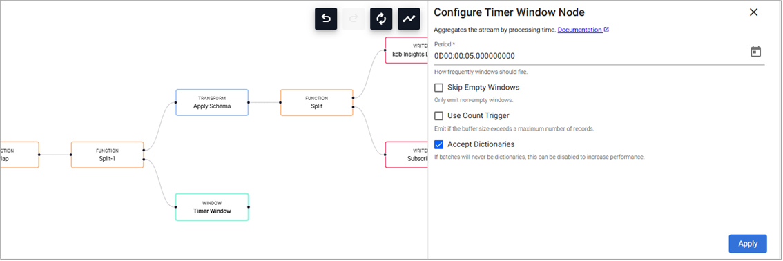
Read more about the Window Timer Windows here.
-
-
Next we define the business logic for the analytic in a Map node.
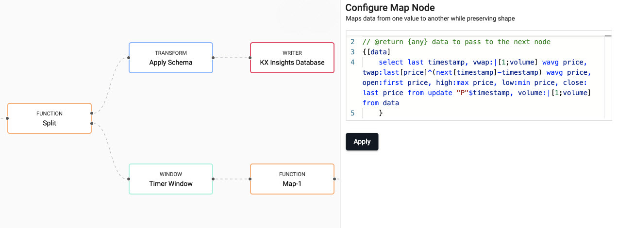
- Add a Map node from the Functions, and connect it to the Timer Window node.
- Click on the Map node and, in the Configure Map Node panel, replace the code displayed with the following code.
// the following code is calculating the fields:
// 1) vwap = weighted average price, adjusted by volume, over a given time
// 2) twap = weighted average price over a given time
// 3) open = price at which a security first trades when an exchange opens for the day
// 4) high = highest price security is traded at
// 5) low = lowest price security is traded at
// 6) close = price at which a security last trades when an exchange closes for the day
// 7) volume = volume of trades placed
{[data]
    select last timestamp,
    vwap:|[1;volume] wavg price,
    twap:last[price]^(next[timestamp]-timestamp) wavg price,
    open:first price,
    high:max price,
    low:min price,
    close: last price
    from update "P"$timestamp,
        volume:|[1;volume]
    from data
    }
kdb+/q functions explained
If any of the above code is new to you don't worry, we have detailed the q functions used above:
-
Click Apply.
-
Next, the data generated by the analytic must be transformed into a format a streaming subscriber can understand.
- Add an Apply Schema node to the pipeline workspace and connect it to the Map-1 function node.
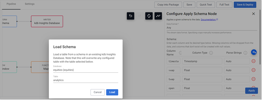
- Click on the Apply Schema-1 node and, in the Configure Apply Schema Node panel, click the Load Schema icon.
- Select equities (equities) as the database and analytics as the table and click Load.
- Click Apply
-
-
Add a Subscriber node to the pipeline.
-
Connect the Apply Schema-1 node to the Subscriber node.
-
Define the following settings to the Subscriber-1 node:
Setting Value Details table analytics The identifier used by the View to access the data. Publish Frequency 100 How regularly the subscriber updates the web-socket in milliseconds. Snapshot Cache Limit 100 How many rows of data is cached on the Subscriber node for use when the View loads the data. -
Click Apply to apply these settings.
-
-
Next, the results of the VWAP analytic must be stored to the database.
Note
This step is optional for streaming the results to the view, but it is useful to write the results to the database for historical viewing.
-
From the pipeline template view, add a Split node from the list of Function nodes.
- Right-click the link between the Apply Schema-1 and Subscriber-1 nodes, and click Delete Edge.
- Connect the left hand point-edge of the Split-2 node to the Apply Schema-1 node.
- Connect the first point-edge of the Split-2 node to the Subscriber-1 node.
-
Add a kdb Insights Database writer node to the pipeline workspace.
- Connect the first point-edge of the Split-2 node to the kdb Insights Database-1 node.
- Click on the kdb Insights Database-1 node and, in the Configure kdb Insights Database Node panel select equities (equities) as the database and analytics as the table.
- Click Apply
-
-
Click Save.
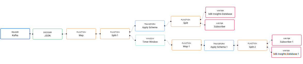
The workflow now looks like the following:
-
Deploy the package:
- Click on Packages, in the left-hand menu to open the Packages index.
-
Click on the three dots to the right of the equities package and click Deploy.
The Deploy Package dialog open. Click Deploy.
To load and review the ready-made view
-
Click + on the ribbon menu and choose View to open the Create View screen.
- Set the View Name to equities-tmp.
- From the Select a package drop-down, choose equities.
- Click Create.
-
Upload the ready-made View:
- Click here to display a JSON representation of the ready-made Equities View in a new browser window.
- Select all the text in the new browser window and copy it into an empty text file using the editor of your choice.
- Save the file on your machine. The file must be saved with a .json extension.
- Drag the file over the View, going to the top left-hand corner. When the workspace is highlighted in blue and Drop Dashboards to Import is displayed in the center of the workspace you can drop the file.
In the Create View dialog set the following:
Setting Value View Name equities Select a Package equities -
Click Create
The View is displayed.
Note
You can delete the equities-tmp view now the actual equities View has been imported.
-
Click Preview to view the charts. Here you can see that the charts use both live and historic data for the big picture in the market.
The chart, in the top of the View, S&P Intraday, streams the price data and VWAP analytic generated by the equities-1 pipeline. This is a live feed of price and the calculated VWAP analytic.
The chart, in the lower part of the View, Daily Price Asset plots historic index data ingested by the Amazon S3 object storage pipeline. This is a time series chart of historic index data.
The following screenshot shows the new View.
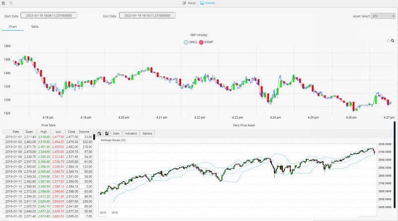
Access the Equities view from the left-hand menu of the Overview page. The top chart is a live feed of price and the calculated VWAP analytic. The lower chart is a time series chart of historic index data.
-
The Price Table tracks positions in the market.
In the top chart, a green highlight is used if a Long (a buyer) trade, or red if Short (a seller).
A similar highlight is used in the table on the left and in the volume bars of the lower chart.
Next steps
- Learn how to build and run a machine learning model to create stock predictions in real-time on this financial dataset in the next tutorial.
- Learn more about how to use kdb Insights Enterprise by following our other guided walkthroughs.
Further reading
- Web interface overview explaining the functionality of the web interface
- Create & manage databases to store data
- Create & manage pipelines to ingest data
- Create & manage queries to interrogate data
- Create & manage views to visualize data