Manufacturing - Real-Time Fault Prediction
This page provides a tutorial on how compute logic can be applied to live data streaming from a MQTT messaging service. It then uses Deep Neural Network Regression to determine the likelihood of breakdowns.
For manufacturers, machine downtime can cost millions of dollars a year in lost profits, repair costs, and lost production time for employees. By embedding predictive analytics in applications, such as kdb Insights Enterprise, manufacturing managers can monitor the condition and performance of assets and predict failures before they happen.
Benefits
This tutorial highlights the following benefits of using kdb Insights Enterprise:
| benefit | description |
|---|---|
| Predictive analysis | Predictive analytics and data visualizations enable you to forecast a view of asset health and reliability performance. |
| Reduce risks | Leverage data in real time for detection of issues with processes and equipment, reducing costs and maximizing efficiencies throughout the supply chain with less overhead and risk. |
| Control logic | Explore how to rapidly develop and visualize computations to extract insights from live streaming data. |
This tutorial explains how to build an intelligent data pipeline, by creating a database to store incoming data. It them explains how to ingest live MQTT data into the database to enable real-time analytics. Once the data is available, you can query the data to explore its structure and assess its quality. Based on the insights, you are shown how to define a standard compute logic to preprocess and transform the data into a suitable format. Then, you can apply a deep neural network regression model to derive predictive insights. Finally, you can query the model to retrieve predictions and evaluate the model's performance within the pipeline.
Create a database
-
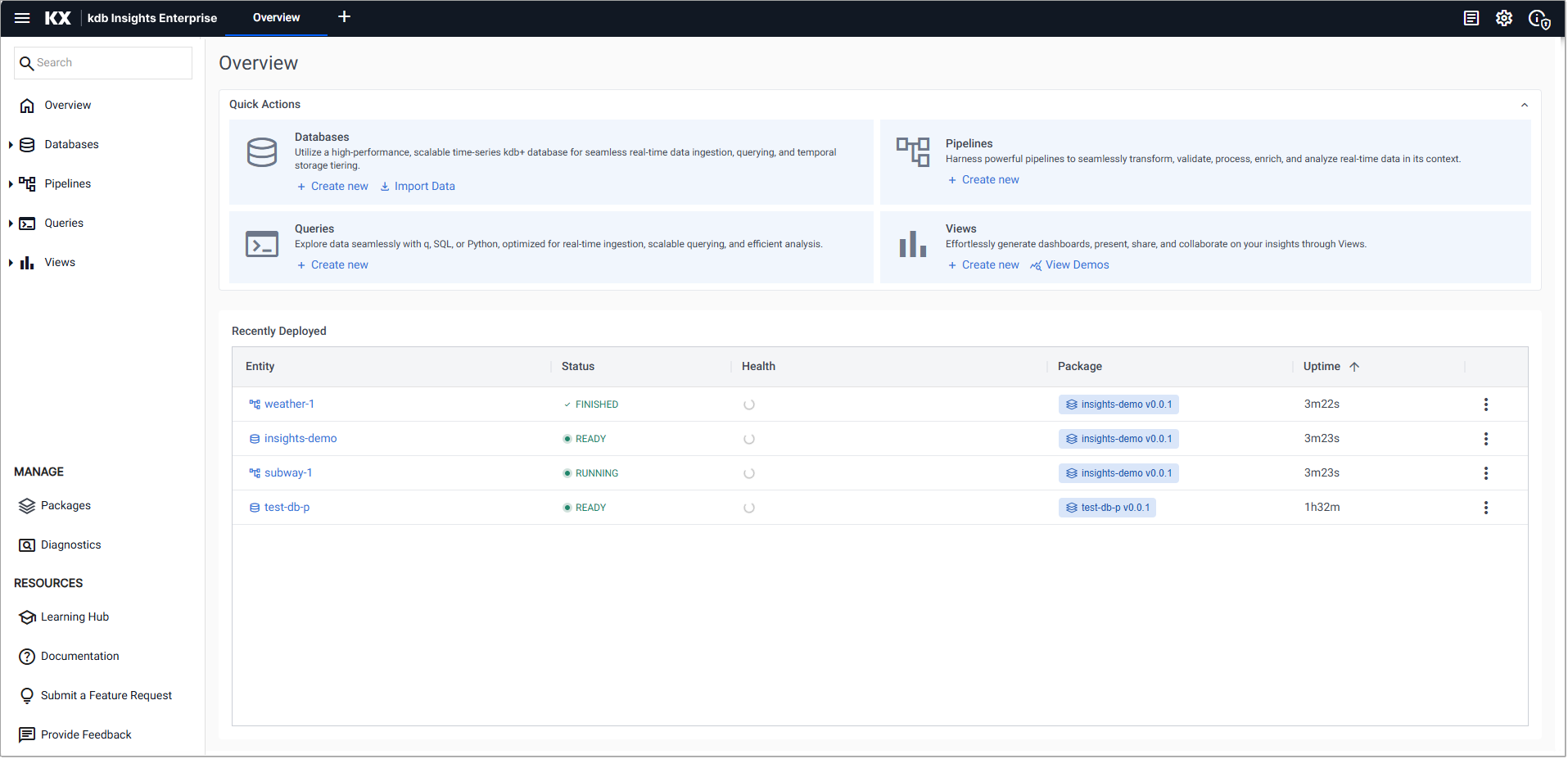
Click Create new under Databases on the Overview page.
-
In the Create Database dialog set the following:
-
Click Create
-
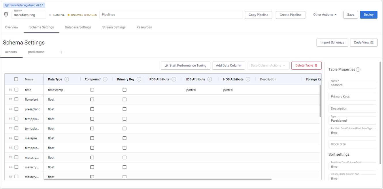
On the Schema Settings tab, click Code View, on the right-hand side, and replace the code displayed with the following JSON:
Manufacturing JSON schema
Paste into the code editor:
[ { "name": "sensors", "type": "partitioned", "primaryKeys": [], "prtnCol": "time", "sortColsDisk": [ "time" ], "sortColsMem": [ "time" ], "sortColsOrd": [ "time" ], "columns": [ { "type": "timestamp", "attrDisk": "parted", "attrOrd": "parted", "name": "time", "attrMem": "" }, { "name": "flowplant", "type": "float", "attrMem": "", "attrOrd": "", "attrDisk": "" }, { "name": "pressplant", "type": "float", "attrMem": "", "attrOrd": "", "attrDisk": "" }, { "name": "tempplantin", "type": "float", "attrMem": "", "attrOrd": "", "attrDisk": "" }, { "name": "tempplantout", "type": "float", "attrMem": "", "attrOrd": "", "attrDisk": "" }, { "name": "massprecryst", "type": "float", "attrMem": "", "attrOrd": "", "attrDisk": "" }, { "name": "tempprecryst", "type": "float", "attrMem": "", "attrOrd": "", "attrDisk": "" }, { "name": "masscryst1", "type": "float", "attrMem": "", "attrOrd": "", "attrDisk": "" }, { "name": "masscryst2", "type": "float", "attrMem": "", "attrOrd": "", "attrDisk": "" }, { "name": "masscryst3", "type": "float", "attrMem": "", "attrOrd": "", "attrDisk": "" }, { "name": "masscryst4", "type": "float", "attrMem": "", "attrOrd": "", "attrDisk": "" }, { "name": "masscryst5", "type": "float", "attrMem": "", "attrOrd": "", "attrDisk": "" }, { "name": "tempcryst1", "type": "float", "attrMem": "", "attrOrd": "", "attrDisk": "" }, { "name": "tempcryst2", "type": "float", "attrMem": "", "attrOrd": "", "attrDisk": "" }, { "name": "tempcryst3", "type": "float", "attrMem": "", "attrOrd": "", "attrDisk": "" }, { "name": "tempcryst4", "type": "float", "attrMem": "", "attrOrd": "", "attrDisk": "" }, { "name": "tempcryst5", "type": "float", "attrMem": "", "attrOrd": "", "attrDisk": "" }, { "name": "temploop1", "type": "float", "attrMem": "", "attrOrd": "", "attrDisk": "" }, { "name": "temploop2", "type": "float", "attrMem": "", "attrOrd": "", "attrDisk": "" }, { "name": "temploop3", "type": "float", "attrMem": "", "attrOrd": "", "attrDisk": "" }, { "name": "temploop4", "type": "float", "attrMem": "", "attrOrd": "", "attrDisk": "" }, { "name": "temploop5", "type": "float", "attrMem": "", "attrOrd": "", "attrDisk": "" }, { "name": "setpoint", "type": "float", "attrMem": "", "attrOrd": "", "attrDisk": "" }, { "name": "contvalve1", "type": "float", "attrMem": "", "attrOrd": "", "attrDisk": "" }, { "name": "contvalve2", "type": "float", "attrMem": "", "attrOrd": "", "attrDisk": "" }, { "name": "contvalve3", "type": "float", "attrMem": "", "attrOrd": "", "attrDisk": "" }, { "name": "contvalve4", "type": "float", "attrMem": "", "attrOrd": "", "attrDisk": "" }, { "name": "contvalve5", "type": "float", "attrMem": "", "attrOrd": "", "attrDisk": "" } ] }, { "columns": [ { "type": "timestamp", "attrDisk": "parted", "attrOrd": "parted", "name": "time", "attrMem": "" }, { "name": "model", "type": "symbol", "attrMem": "", "attrOrd": "", "attrDisk": "" }, { "name": "prediction", "type": "float", "attrMem": "", "attrOrd": "", "attrDisk": "" } ], "primaryKeys": [], "type": "partitioned", "prtnCol": "time", "name": "predictions", "sortColsDisk": [ "time" ], "sortColsMem": [ "time" ], "sortColsOrd": [ "time" ] } ] -
Click Apply.
-
Click Save.
- Click Deploy, and in the database resources dialog click Deploy again.
-
Click the arrow on the Databases menu, on the left-hand panel, to display the list of databases. When a green tick is displayed beside the manufacturing database the database is ready to use.

Setting Value Database Name manufacturingSelect a Package Create new packagePackage Name manufacturing-db-pkg
Database warnings
Once the database is active, warnings are displayed in the Issues pane of the Database Overview page. These are expected and can be ignored.
Ingest live MQTT data
MQTT is a standard messaging protocol used in a wide variety of industries, such as automotive, manufacturing, telecommunications, oil and gas, etc.
-
On the Overview page, in the Quick Actions panel under Databases, in the Quick Actions panel.
-
In the Import your data screen click MQTT.
-
In the Configure MQTT screen, complete the properties:
Setting Value Broker ssl://mqtt.insights-data.kx.com:1883Topic livesensorUsername demoUse TLS disabled -
Click Next.
-
In the Select a decoder screen click JSON.
-
In the Configure JSON screen leave the Decode Each option unchecked, and click Next.
-
In the Configure Schema screen:
-
Leave the Data Format setting set to Any
-
Click the
 icon and apply the following settings:
Setting Value Database manufacturingTable sensors-
Click Load
-
Click Next
-
-
In the Configure Writer screen apply the following settings:
Setting Value Database manufacturing (manufacturing-db-pkg)Table sensorsLeave the remaining fields unchanged:
Setting Value Write direct to HDB unchecked Deduplicate Stream unchecked Set Timeout Value unchecked -
Click Create Pipeline to display the Create Pipeline dialog.
Setting Value Database Name manufacturing-mqttSelect a Package Create new packagePackage Name manufacturing-pipelinesThe database and pipeline should be in different packages.
Click Create once you've configured the settings above. This opens a new tab where you can configure your pipeline.
-
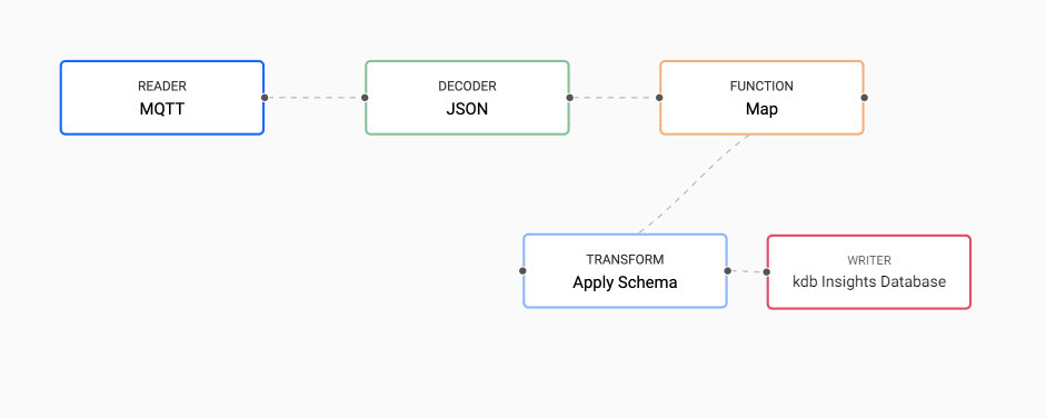
In the Pipeline tab, right-click the link between the Decoder and Transform nodes, and click Delete Edge to remove.
-
Drag a Map node from the Functions category on the left-hand side into the pipeline layout.
-
Connect the Map node to the Decoder and Transform nodes with a click-and-drag connect of the dot edge of the node.
-
Click on the Map node and in the Configure Map Node panel, replace the q code with the following. enlist transforms the kdb+ dictionary to a table.
{[data] enlist data } -
Click Apply in the Configure Map Node panel.
-
Go to the Settings tab. Under Environment Variables & Secrets, add the variable
KXI_ALLOW_NONDETERMINISMand set its value totrue.Note
The MQTT reader requires this setting because it operates in a non-deterministic manner. In addition, deduplication for the database writer was disabled earlier, as deduplication requires deterministic processing.
-
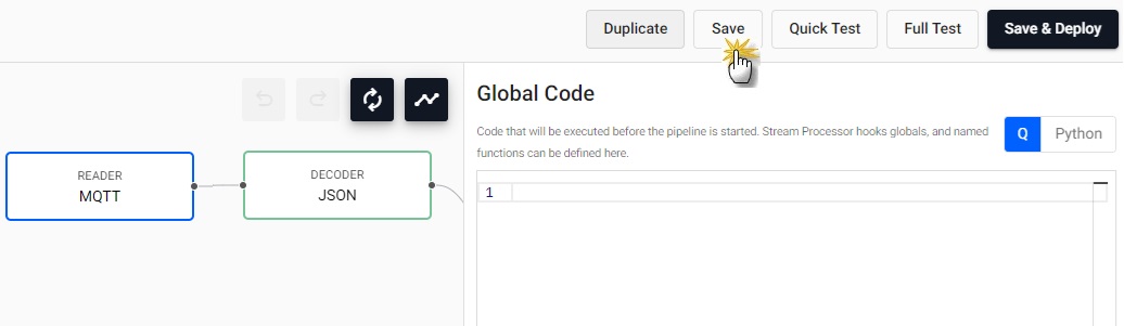
Return to the Editor tab and click Save & Deploy.
-
In the Enter Password for MQTT dialog enter
demoand click OK.Deploying a pipeline requires an active database to receive the data. Ensure the manufacturing database is deployed and active before deploying the
MQTTpipeline. This is the last step in the previous section. -
Go to the Running Pipelines section on the Overview page. When the Status of manufacturing-mqtt = Running it is ready to be queried.
Query the data
To query the MQTT data:
-
Click + on the ribbon menu, and click Query.
-
In the Query & Load Data panel, click on the SQL tab.
Allow 15-20 minutes of data generation before querying the data. Certain queries may return visuals with less data if run too soon.
-
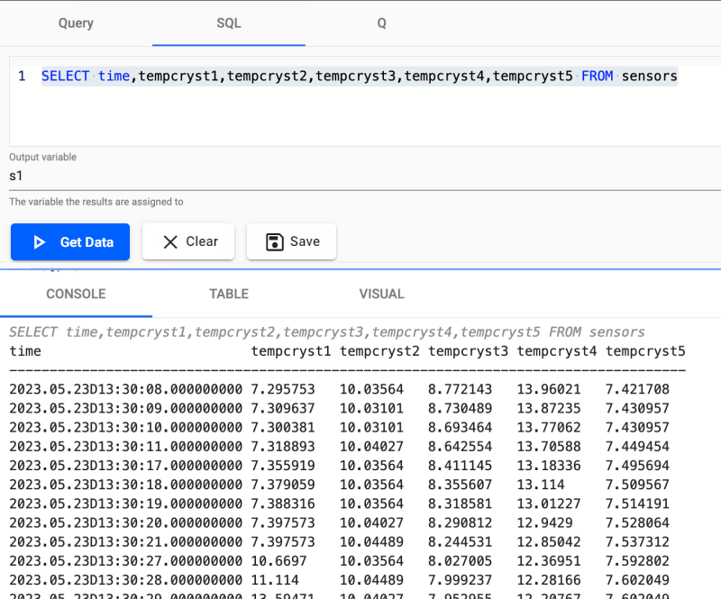
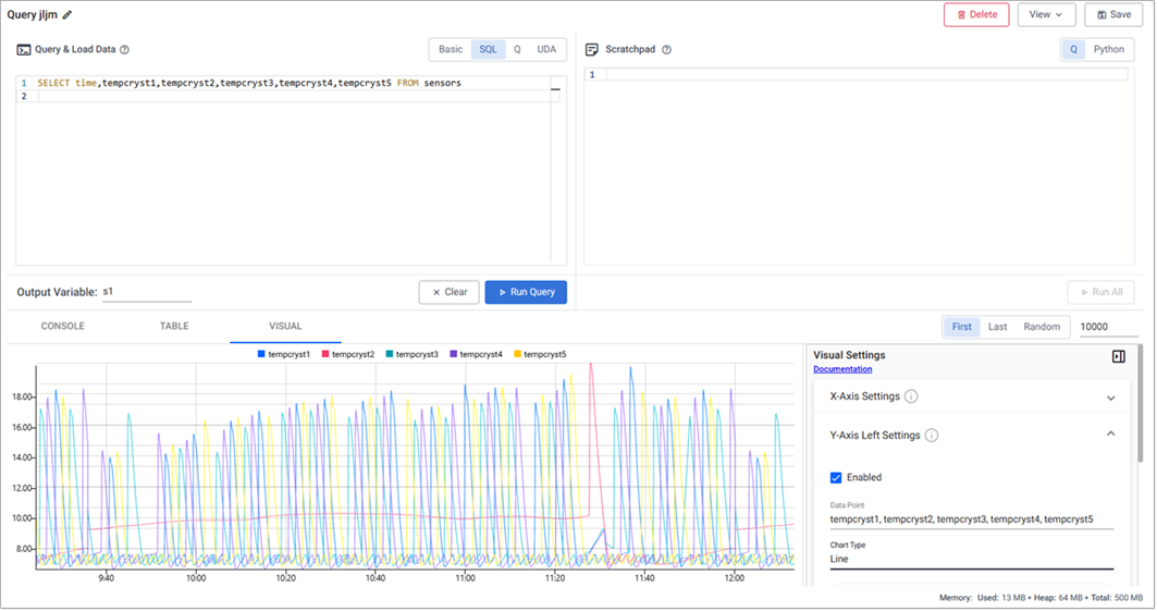
After clicking on the SQL tab, copy and paste the following code:
SELECT time,tempcryst1,tempcryst2,tempcryst3,tempcryst4,tempcryst5 FROM sensors -
Enter s1 as the Output variable.
-
Click Run Query to generate the results.
-
Click on the Visual tab, and click Run Query again.
-
In the Y-Axis Left Settings select Line as the Chart Type .
In following screenshot, there is a cyclical pattern of temperature in the crystallizers, fluctuating between 7-20 degrees Celsius.
-
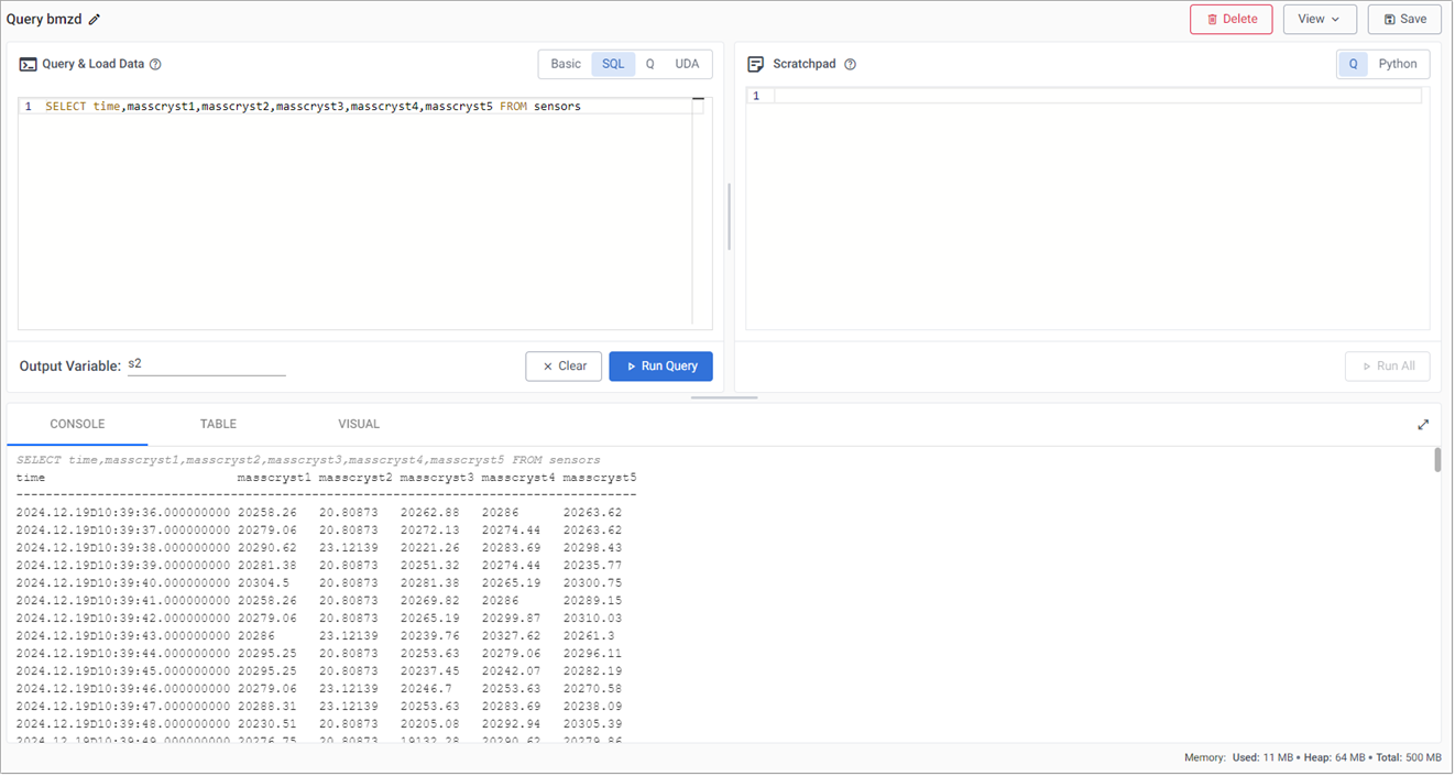
You can also query data for the mass fields using SQL. Similar fluctuations to those for the temperature values occur for mass levels in the crystallizers, moving between 0-20000kg on a cycle.
-
Replace the query in the SQL tab with the following:
SELECT time,masscryst1,masscryst2,masscryst3,masscryst4,masscryst5 FROM sensors -
Change the Output variable to s2.
-
Click Run Query.
-
Define a standard compute logic
In this section we use the scratchpad to set Control Chart Limits to identify predictable Upper Control (UCL) and Lower Control Limits (LCL).
This section describes how to calculate a 3 sigma UCL and LCL to account for 99.7% of expected temperature fluctuations. A recorded temperature outside of this range requires investigation.
-
Copy and paste the code below into the Scratchpad panel on the right.
// Calculating 5 new values, most notably ucl and lcl where
// ucl - upper control limit
// lcl - lower control limit
select lastTime:last time,
    lastVal: (1.0*last tempcryst3),
    countVal: count tempcryst3,
    ucl: avg tempcryst3 + (3*dev tempcryst3),
    lcl: avg tempcryst3 - (3*dev tempcryst3)
    by xbar[10;time.minute]
    from s1
q/kdb+ functions explained
For more information on the code elements used in the above query:
-
Click Run All.
-
Visualize the threshold by selecting the Line graph. The change in control limits is more obvious in the visual similar to the graph below after ~15-20 minutes of loading data.
This shows a plot of a 3 sigma upper and lower control temperature bound to account for 99.7% of expected temperature fluctuation in manufacturing process. Outliers outside of this band require investigation.
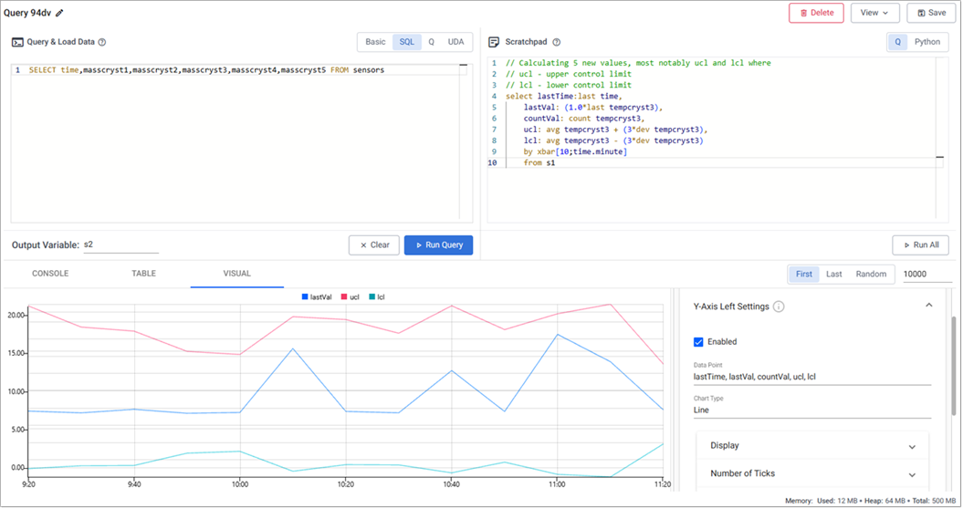
Plot of a 3 sigma upper and lower control temperature bound to account for 99.7% of expected temperature fluctuation in manufacturing process; outliers outside of this band require investigation.
-
-
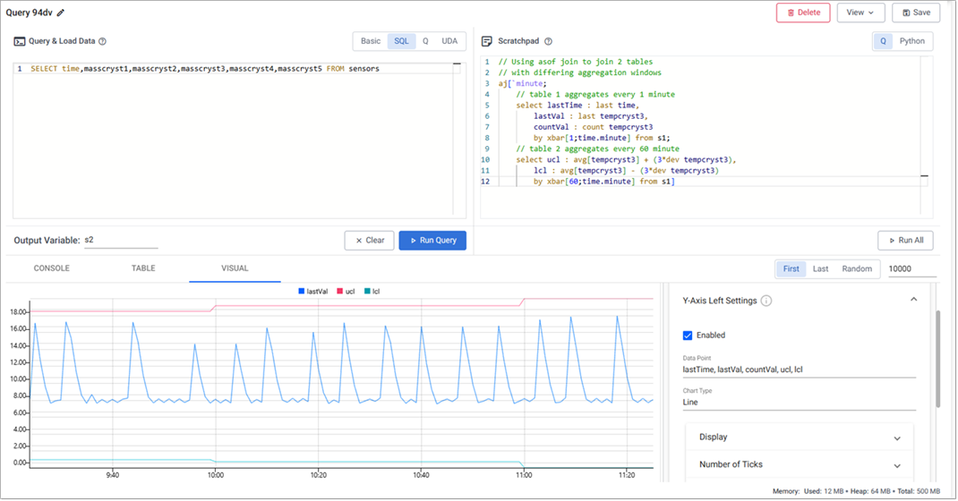
Next, aggregate temperature thresholds over two rolling time windows; a 1 minute aggregate and a second, smoother, 60 minute aggregate of sensor readings.
-
Replace all code in the scratchpad with the code below:
// Using asof join to join 2 tables
// with differing aggregation windows
aj[`minute;
    // table 1 aggregates every 1 minute
    select lastTime : last time,
        lastVal : last tempcryst3,
        countVal : count tempcryst3
        by xbar[1;time.minute] from s1;
    // table 2 aggregates every 60 minutes
    select ucl : avg[tempcryst3] + (3*dev tempcryst3),
        lcl : avg[tempcryst3] - (3*dev tempcryst3)
        by xbar[60;time.minute] from s1]
q/kdb+ functions explained
For more information on the code elements used in the above query:
aj is a powerful timeseries join, also known as an asof join, where a time column in the first argument specifies corresponding intervals in a time column of the second argument.
This is one of two bitemporal joins available in kdb+/q.
To get an introductory lesson on bitemporal joins, view the free Academy Course on Table Joins.
-
Click Run All to view a plot of aggregate temperature thresholds for 1 minute and 60 minutes.
-
-
Next, define a function to simplify querying and run the query with a rolling 1 minute window:
-
Append the code below to the code already in the scratchpad:
// table = input data table to query over
// sd = standard deviations required
// w1 = window one for sensor readings to be aggregated by
// w2 = window two for limits to be aggregated by
controlLimit:{[table;sd;w1;w2]
    aj[`minute;
    // table 1
    select lastTime : last time,
        lastVal : last tempcryst3,
        countVal : count tempcryst3
        by xbar[w1;time.minute] from table;
    // table 2
    select ucl : avg[tempcryst3] + (sd*dev tempcryst3),
        lcl : avg[tempcryst3] - (sd*dev tempcryst3)
        by xbar[w2;time.minute] from table]
    }

controlLimit[s1;3;1;60]
q/kdb+ functions explained
For more information on the code elements used in the above query:
{} known as lambda notation allows us to define functions.
It is a pair of braces (curly brackets) enclosing an optional signature (a list of up to 8 argument names) followed by a zero or more expressions separated by semicolons.
To get an introductory lesson, view the free Academy Course on Functions.
-
Click Run All.
-
-
Finally, change the
w1parameter value to see the change in signal when you use different window sizes:-
Append the code below to the code already in the scratchpad, to set the parameter to 10 minutes:
controlLimit[s1;3;10;60] -
Append the code below to the code already in the scratchpad, to set the parameter to 20 minutes:
controlLimit[s1;3;20;60]
By varying the parameter for one of the windows, you can see the change in signal between rolling windows of 1, 10 and 20 minutes. This means you can tailor the output to make it smooth as per your requirements.
-
Apply a deep neural network regression model
Apply a trained neural network model to incoming data. The architecture of a neural network regression model as it relates to kdb Insights Enterprise is shown here.
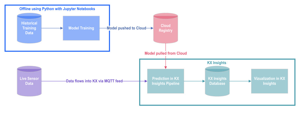
For this use case, our model is pre-trained using tensorflow neural networks and xgboost. Each model prediction is then aggregated for added benefit.
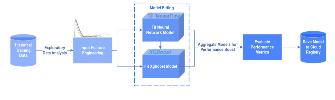
kdb Insights Enterprise offers a range of machine learning nodes in the pipeline template to assist in model development.
- Click on the arrow to the left of Pipelines in the left-hand menu and click on manufacturing-mqtt to open the pipeline screen, or click on the Pipeline tab if it's still open.
- Click Copy into Package.
- Update the name to manufacturing-ml
- Click Select a Package and choose manufacturing-pipelines.
-
Click Create.
-
In the manufacturing-ml pipeline screen, paste the following code in the Global Code panel. Copy either the q or Python code, as relevant to your specific case.
ewmaLag100:0n;
ewmaLead100:0n;
ewmaLag300:0n;
ewmaLead300:0n;
timeSince:0n;
started:0b;
back:0n;
import numpy as np import pykx as kx ewmaLag100 = np.nan ewmaLead100 = np.nan ewmaLag300 = np.nan ewmaLead300 = np.nan timeSince = np.nan started = False back = np.nan -
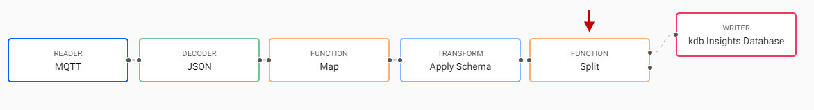
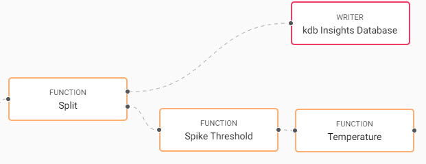
Drag a Split Function node to the pipeline.
This split maintains the original database write as one path, and adds the machine learning workflow to the second path.
- Right-click the existing link between the Apply Schema and kdb Insights Database node, and click Delete Edge.
- Position the Split node between the Apply Schema and kdb Insights Database node.
- Connect the Split node to the Apply Schema and kdb Insights Database node with a click-and-drag connect of the dot edge of the node.
-
Drag a Map Function node onto the pipeline.
-
Connect the Split node to the Map node.
-
Click on the Map node and copy and replace the existing code with the following to the code editor using either Python or Q tab, leave Allow Partials checked:
{[data]
    data:-1#data;
    $[(first[data[`masscryst3]]>1000)&(not null back)&(back<1000);
    [timeSince::0;
        back::first[data[`masscryst3]];
        tmp:update timePast:timeSince from data];
    [timeSince::timeSince+1;
        back::first[data[`masscryst3]];
        tmp:update timePast:timeSince from data]
    ];
    select time,timePast,tempcryst4,tempcryst5 from tmp
}
def func(data):
    global timeSince, back
    if (data["masscryst3"][0].py()>1000)&(not np.isnan(back))&(back < 1000):
        timeSince = 0.0
    else:
        timeSince = timeSince + 1.0

    back = data["masscryst3"][0].py()
    d = data.pd()
    d['timePast'] = timeSince
    return d[['time','timePast','tempcryst4','tempcryst5']]
This adds a new variable, timePast, that calculates the time interval between spikes. A spike occurs when product mass breaks above the spike threshold of 1,000 kg.
-
Click Apply.
-
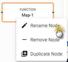
Right-click on the Map-1 node and Rename Node to Spike Threshold. Click OK.
-
Drag a third Map Function node onto the pipeline.
-
Connect it to the Spike Threshold node.
-
Click on the new Map-1 node, and in either the Python or Q tab of the Configure Map Node panel replace the existing code with the following. Leave Allow Partials checked:
{[data]
    a100:1%101.0;
    a300:1%301.0;
    $[not started;
    [ewmaLag100::first data`tempcryst5;
    ewmaLead100::first data`tempcryst4;
    ewmaLag300::first data`tempcryst5;
    ewmaLead300::first data`tempcryst4;
    started::1b];
    [ewmaLag100::(a100*first[data[`tempcryst5]])+(1-a100)*ewmaLag100;
    ewmaLead100::(a100*first[data[`tempcryst4]])+(1-a100)*ewmaLead100;
    ewmaLag300::(a300*first[data[`tempcryst5]])+(1-a300)*ewmaLag300;
    ewmaLead300::(a300*first[data[`tempcryst4]])+(1-a300)*ewmaLead300
    ]];
    t:update ewmlead300:ewmaLead300,ewmlag300:ewmaLag300,ewmlead100:ewmaLead100,ewmlag100:ewmaLag100 from data;
    select from t where not null timePast
}
def func(data): global started,ewmaLag100,ewmaLead100,ewmaLag300,ewmaLead300 a100=1/101.0 a300=1/301.0 if not started: started = True ewmaLag100 = data["tempcryst5"][0].py() ewmaLead100 = data["tempcryst4"][0].py() ewmaLag300 = data["tempcryst5"][0].py() ewmaLead300 = data["tempcryst4"][0].py() else: ewmaLag100 = a100*data["tempcryst5"][0].py() + (1-a100)*ewmaLag100 ewmaLead100 = a100*data["tempcryst4"][0].py() + (1-a100)*ewmaLead100 ewmaLag300 = a300*data["tempcryst5"][0].py() + (1-a300)*ewmaLag300 ewmaLead300 = a300*data["tempcryst4"][0].py() + (1-a300)*ewmaLead300 d = data.pd() d['ewmlead300'] = ewmaLead300 d['ewmlag300'] = ewmaLag300 d['ewmlead100'] = ewmaLead100 d['ewmlag100'] = ewmaLag100 d['model'] = kx.SymbolAtom("ANN") d = d[~(np.isnan(d.timePast))] return dThis calculates moving averages for temperature.
-
-
Click Apply.
-
Right-click on the Map-1 node and Rename Node to Temperature. Click OK.
-
Connect the Spike Threshold node to the Temperature node.
-
Drag the Predict Using Registry Model, Machine Learning node onto the pipeline.
-
Connect it to the Temperature node.
-
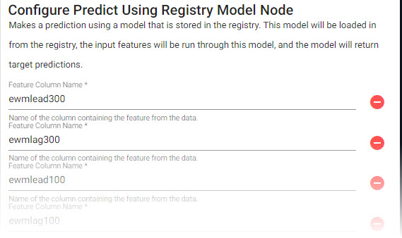
Click on the ML node and in the Configure Predict Using Registry Model Node tab click + to add each if the following Feature Column Name.
- ewmlead300
- ewmlag300
- ewmlead100
- ewmlag100
- tempcryst4
- tempcryst5
- timePast
-
Set the remaining properties as follows:
setting value Prediction Column Name yhat Registry Type AWS S3 Registry Path s3://kxs-prd-cxt-twg-roinsightsdemo/qrisk
-
Click Apply.
-
Drag another Map Function node onto the pipeline.
-
Connect it to the Machine Learning node.
-
Click on the new Map node, and in the Configure Map Node panel, copy and paste the following into either the Python or Q tab. Leave Allow Partials checked:
{[data]
    select time, model:`ANN, prediction:"f"$yhat from data
}
def func(data): d = data.pd() d['prediction'] = d['yhat'].astype(float) return d[['time','model','prediction']]This adds some metadata.
- Click Apply.
-
Right-click on the Map node and Rename Node to Metadata. Click OK.
-
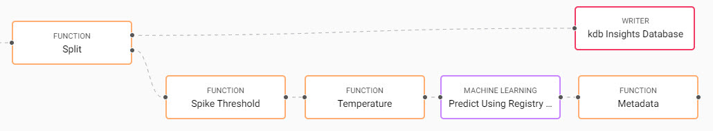
Drag a second kdb Insights Database Writer node onto the pipeline.
-
Connect this to the Metadata node.
-
Apply the following settings:
Setting Value Database manufacturing Table predictions Write direct to HDB Unchecked Deduplicate Stream Unchecked Set Timeout Value Unchecked
This completes the workflow and writes the predictions to the predictions table.
- Click Apply.
-
-
Click on the Settings tab in pipeline.
-
Scroll down to the Environment Variables, click + Add Variable to add the following:
Variable Value Description AWS_REGION eu-west-1 This variable provides the region details that are required to access the machine learning model on AWS cloud storage. KX_KURL_DISABLE_AUTO_REGISTER 1 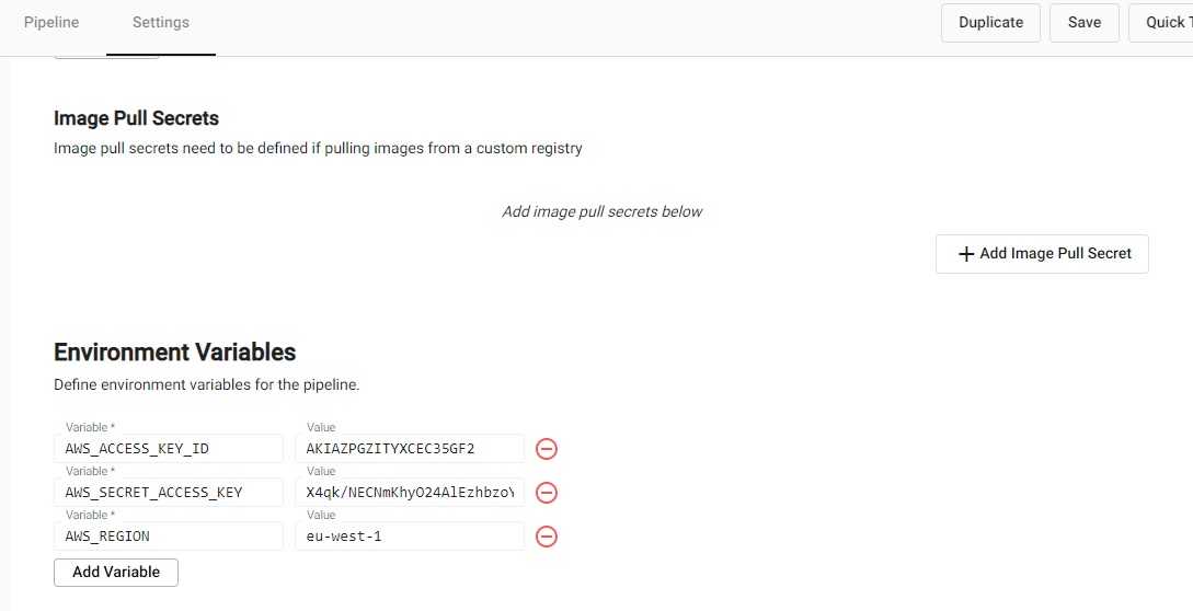
-
Click Save.
-
Go to the Overview page, and if the manufacturing-mqtt pipeline is running, click on the X and click Teardown and select Clean up resources after teardown and click Teardown Pipeline.
-
Click on manufacturing-ml under Pipelines on the left-hand menu and click on Save & Deploy.
-
In the Enter Password for MQTT dialog, enter demo and click OK.
-
On the Overview page in the Running Pipelines panel, when the Status of manufacturing-ml is Running the prediction model has begun.
-
Next, you can query the model, as described in the next section.
Query the model
It takes at least 20 minutes to calculate the timePast variable as two spikes are required. For more spikes in the data, shorten the frequency of spike conditions.
After sufficient time has passed, click + on the ribbon menu and click Query.
-
In the Query & Load Data panel, Basic tab, define the values:
Setting Value Table name predictionsOutput variable p1 -
Select the Visual tab.
-
Click Run Query.
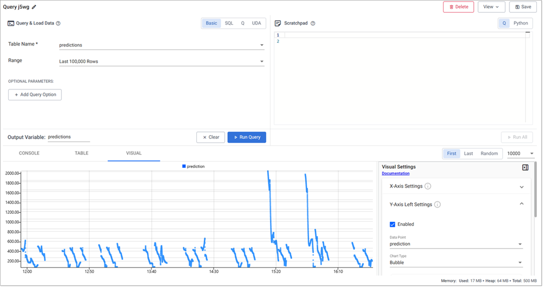
-
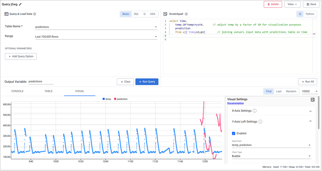
Compare the prediction to real-world data;
-
In the scratchpad paste the following:
select time, temp:20*tempcryst4, // adjust temp by a factor of 20 for visualization purposes prediction from aj[`time;s1;p1] // joining sensors input data with predictions table on time -
Click Run All.
-
Summary
The red predictive data aligns closely with the real-world data shown in blue, demonstrating strong model potential. With additional data, the model performance is expected to improve further.
The prediction model gives the manufacturer advance notice to when a cycle begins and expected temperatures during the cycle. Such forecasting informs the manufacturer of filtration requirements.
In a typical food processing plant, levels can be adjusted relative to actual temperatures and pressures. By predicting parameters prior to filtration, the manufacturer can alter rates in advance, thus maximizing yields.
This and other prediction models can save millions of dollars in lost profits, repair costs, and lost production time for employees. By embedding predictive analytics in applications, manufacturing managers can monitor the condition and performance of assets and predict failures before they happen.