Sizing kdb Insights Deployments

This page provides guidance for sizing kdb Insights deployments, including best practices for scaling disks, CPU, and memory for key components.

The infrastructure requirements for a kdb Insights deployment are driven by multiple factors, including:

Data flow: what data is ingested, stored, transformed, streamed
Query workload: complexity and volume of queries

The sections below provide a high-level overview of the key processes and show how sizing them is impacted by factors such as table sizes, shards and late data.

Reference cluster sizes

The following two workload cases illustrate how variations in workload complexity significantly affect cluster sizing.

The light workload case represents a near best-case scenario e.g. little data transformation is required and queries are simple. It reflects more what is possible or ideal rather than what is typical.
The intensive workload case requires much more memory to process the same amount of data. Data transformation is intensive, and queries are complex and many may arrive concurrently. While not a worst-case scenario, it demonstrates the requirements of running a more complex workload.

Cloud and OpenShift

Cloud means AWS, GCP, or Azure. OpenShift clusters are treated separately from cloud-based ones as OpenShift adds substantial sizing overheads. Where N/A appears, it means the node is too small for the deployment.

Light workload

The following table is based on the real-time ingest of a single table with 20 columns per row into a single shard spread over the entire day. It assumes:

low memory usage for pipelines
two Data Access Processes (DAPs) with simple queries
use of Rook-CephFS
no provisioning for Storage Manager (SM) failover

The rows/day figure is based on having three nodes of the listed size ingesting that amount of data in real time.

Node size (GiB)	Rows/day cloud (millions)	GiB/day cloud	Rows/day OpenShift (millions)	GiB/day OpenShift
32	1,400	209	N/A	N/A
64	8,500	1,267	7,100	1,058
96	15,500	2,310	14,200	2,116
128	22,600	3,368	21,300	3,174
192	27,000	4,023	27,000	4,023
256	27,000	4,023	27,000	4,023

Intensive workload

This table is based on two tables in one shard: one real-time with 20 columns and an 8 hour ingest window (e.g. an equities trading day), and one batch-loaded once per day with 50 columns. The ratio of rows in the two tables is 10:1. It assumes:

medium memory usage for pipelines
four DAPs with heavy queries
use of Rook-CephFS
provision of enough memory so the pods on a failing node can be started on the remaining two

The rows/day figure is based on having three nodes of the listed size ingesting that number of real-time rows, with 10% as many batch rows.

Node size (GiB)	Rows/day cloud (millions)	GiB/day cloud	Rows/day OpenShift (millions)	GiB/day OpenShift
32	N/A	N/A	N/A	N/A
64	220	41	130	24
96	520	97	430	80
128	820	153	730	136
192	1,410	263	1,320	246
256	2,000	373	1,920	358

Notes for both tables

Both workloads are based on using two RT clusters with three nodes each.
The ranges shown are guidelines for data ingestion. Capacity within any given band is available for streaming logic, or additional query capacity.
1 GiB stored uncompressed is equivalent to 6.25 million rows in a 20-column table. Compression reduces the size on disk by a factor of 2.5–10x depending on the algorithm and properties of the data.

For more information, refer to Compression Algorithms.
Realistically, for 32 GiB nodes, the default resource requests could be reduced to allow for higher data volume.
The rows/day figure is capped at 27 billion as the SM can't process this table faster than this rate, regardless of memory availability. To achieve higher throughput, split the data across multiple shards.
For very high data rates, keep in mind that VMs have a limit to the total amount of disk that they can access, typically between 250–1000 TiB. This means older data has to be deleted or moved to object storage.

Cluster sizing

The following key components determine both the node sizes and the cluster memory required:

Storage Manager (SM)
Data Access Process (DAP)
Reliable Transport (RT)
Stream Processor (SP)
Aggregators

Additional factors include whether:

Rook-CephFS is used, as this has significant resource requirements (see Database storage classes)
Nodes should be sized to have enough extra capacity to accommodate pods from a failed node (see Failover provision)

Storage Manager (SM)

Each shard includes an SM. It continuously organizes and writes data to disk in small batches, and once per day it constructs a historical database (HDB) partition for the preceding day. These operations can require substantial resources.

Memory factors

End of Interval (EOI) process: requires allocation for a full interval of data of the largest table that is received in real-time. This scales with the length of the EOI interval and the amount of data received during the busiest interval.
End of Day (EOD) process: generally, the EOD process adapts to the available memory. A good guideline is to ensure the SM has at least twice the EOI memory requirement, as other operations run concurrently. However, for tables using a parted attribute, the SM’s memory requirement in bytes is roughly 10 times the number of rows received that day. You can add memory to improve EOD speed.
Batch loading: this can require a substantial amount of memory depending on the schema and attributes. Compared with EOD, batch loading a table and applying the sorted attribute takes roughly 15 times as much memory, while parted uses roughly 12 times as much.

CPU factors

For data rates below 5 MiB/s, EOI and EOD only need 2 or 3 vCPUs apiece.
At higher rates, assign more vCPUs to the SM process.
At very high rates, the EOI process may become a bottleneck. While adding more vCPUs can help, the benefit is limited by the number of columns in the main tables as one thread is assigned to each column.

For a fixed amount of data, batch processing takes more CPU than EODs.

Disk factors

The disk space used to store a table in kdb Insights is roughly 8 bytes * rows * columns. If compression is applied, this typically reduces the storage needs by a factor between 2.5 and 10.
The whole database requires enough storage for an average day's worth of data multiplied by the number of days to store, plus another 2 days to cover intraday database (IDB) requirements. For example, if an average day uses 50 GiB and 5 years should be stored, then ~90 TiB of disk space is required.
While the SM requires an RT log volume, it generally only needs a few GiB. This is sufficient to cover data received from RT and to store the control signals it publishes back.

Data Access Process (DAP)

DAPs read data that the storage manager has written to disk. Their specific resource requirements include memory, CPU, and network. Encryption at rest has a notable impact on query execution time and, for on-disk queries, memory usage.

Memory factors

Data caching for queries: this is a combination of real-time database (RDB) data prior to the EOI writedown, plus late data. It is approximately 16 bytes × columns × (rows per EOI interval + late data rows) per table.

It is influenced by the pctMemThreshold setting, which defines how much memory the RDB can use for in-memory tables before triggering an unscheduled EOI to write data to disk.
Memory allocation for queries: this depends heavily on the types of queries executed on the DAP. Since queries vary widely, guidance is based on generalized characteristics. The multipliers below assume on-disk data is encrypted:
- Light: queries that cover less than 1 hour of data with one filter, or less than 30 minutes with multiple filters. Require approximately 16 bytes × rows in table.
- Medium: queries that cover less than 12 hours of data with one filter, or less than 6 hours with multiple filters. Require approximately 24 bytes × rows in table.
- Heavy: queries that cover more than 12 hours with multiple filters. Can require 40 bytes (or more) × rows in table.

Optimizing memory based on actual queries

These values should be treated as very rough estimates. We recommend directly measuring the memory used while executing your actual queries to get a better idea of any future needs.

If on-disk data is not encrypted, kdb+ does not need additional memory when reading on-disk columns, drastically reducing the memory requirements compared to the encrypted case. However, if a query creates new columns (e.g. total: price*quantity), then sufficient memory is required to hold the entire column. This can be very substantial for queries spanning long time periods, or for very complex queries, in particular if they involve sorting/grouping.

CPU factors

DAPs benefit from multiple vCPUs but there are diminishing returns beyond 3–4 vCPUs per instance.
Fewer vCPUs can be used for less latency-sensitive use cases.
On-disk encryption does not require extra vCPUs but increases query latency.

Disk factors

The DAPs publish very little to RT, and delete RT log files for received data once they're processed. This doesn't amount to a consequential amount of disk. Typically, a few GiB is sufficient.

Network factors

If the DB is stored on a networked file system like Lustre, data must be transferred between the file server and the DAP’s VM. Additionally, some query patterns may require substantial amounts of data to be sent from the DAPs to aggregators. Network bandwidth usage should be monitored to ensure it doesn’t become a bottleneck for query execution. Query latency will increase before the network bandwidth is maxed out.

Reliable Transport (RT)

The memory requirements and CPUs per RT node are adjustable but shouldn't need to exceed 2–3 GiB and 2.5 vCPUs, regardless of workload. Low data rates such as less than 1 MB/s of data should take less than 1 vCPU and less than 1 GiB.

Topology

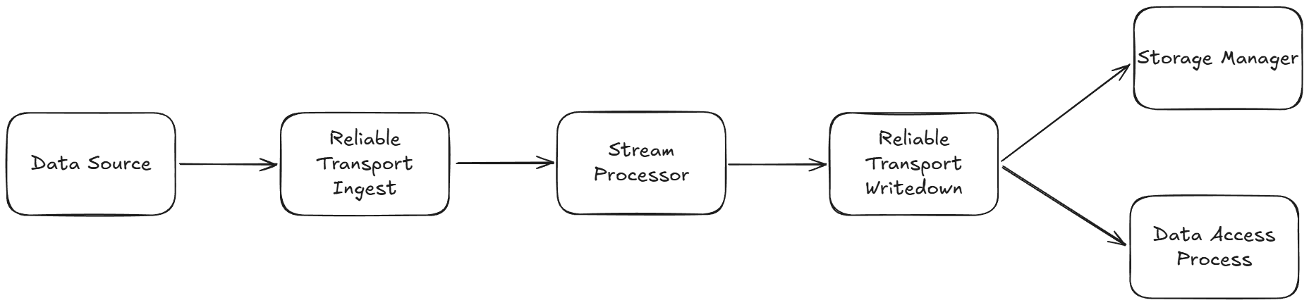
Each assembly typically uses multiple RT nodes for reliability. There are multiple possible configurations. The most general is to have two clusters of three nodes where one cluster is upstream of the SPs and the other is downstream. However, one cluster can cover both the upstream and downstream sides if the set of tables the SP receives are disjointed from those it publishes. Topologically, the two arrangements look like this (simplified to show each cluster rather than individual nodes):

Separate RTs for ingest and writedown

In this topology, the ingest RT cluster is used to ingest the raw data ready for the SP to transform, and the writedown RT cluster contains the data in the right format for writedown:

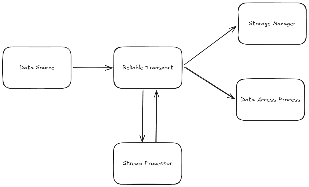
Separate RTs for ingest and writedown

Combined RT for ingest and writedown

In this topology, a single RT cluster is used to transport the raw data to the SP and then subsequently route the transformed, kdb-formatted output to the database components (this requires that input and output table names don't match):

Combined RT

Single node clusters

It's also possible to use a single RT node per cluster e.g. for development systems.

The RT used for data ingestion may not be required where the data source uses a different transport mechanism e.g. Kafka or reading from object storage.

Memory factors

RT memory scales very slowly with overall data volume.

CPU factors

CPU usage scales with total data volume and publish rate. Keep publishes per second below 2,000 by batching rows in the publisher.

Disk factors

Storage needs to scale linearly with the number of days of retention needed, to ensure no data loss in the event that there is a data flow interruption in the system. For more information, see RT Archival.
RT Ingest: more disk is required when the data is in a text format rather than binary. If the data is compressed, this also reduces disk needs. In a typical setup, there are 3 RT nodes, and each needs its own storage. A rough rule of thumb is that each node needs storage at least equal to the size of data it receives over a day times the number of days of retention required to protect against data loss.
RT Writedown: if the SP publishes many rows of data at a time rather than small amounts, it may compress the data before sending it. The threshold for this is triggered when the batch is greater than 2 kB in size. This reduces the disk space consumed by RT Writedown. If the SP drops columns, filters rows, or publishes aggregations of inbound data, this also reduces disk requirements for RT Writedown. The same general guidelines for disk provisioning apply as with RT Ingest.
If using a combined RT setup, disk requirements are reduced to the maximum of the combined inbound and outbound data volumes. This is because if data flow is blocked at some point in the system, disk space is only required for the instance prior to that point. In this case, the combined RT stores all incoming data but doesn't need to store the SP's outgoing messages, as the SP isn't sending anything.

Network factors

In a resilient RT setup with high availability and fault tolerance, the data source streams its data independently to each of the three RT Ingest nodes in the cluster. They replicate the data among themselves for verification, then SP subscribes to each node. As with the data publisher, the SP sends the data to each of the three RT Writedown nodes in the cluster, and the SM and each DAP subscribes to each node. Where the network is a bottleneck, it is possible to reduce the bandwidth needs of the system by configuring publishers to send their data to only one downstream RT node. This comes at the cost of reduced responsiveness if an RT node fails, as the publisher requires a short time to start publishing to one of the remaining RT nodes. For more information, see Alternative topology.
In non-critical environments, a single RT node may be used. This substantially reduces bandwidth requirements but can lead to large delays if the node fails while a new one is started. For more information, see RT Architecture.

Stream Processor (SP)

A shard can have one or more pipelines, each of which may have multiple workers, each using one or more threads. Light workloads may need no more than one single-threaded worker with 0.5 GiB of memory. KX has verified the SP at 3 GiB of RAM under heavy workloads. However, as memory usage is so workload-dependent, the pipeline’s allocation should be set conservatively high initially and later adjusted to match observed usage.

Memory factors

Real-time: data caching, windowing, time bucketing.
Batch: if reading a large file, chunking should be employed to avoid pulling the whole thing into memory.

CPU factors

Logic complexity, including any decoding from a non-kdb format.
Messages per second received/sent (smaller batches at a higher frequency means less scope for vector processing).

Disk factors

Inbound: if receiving data from RT, the v2 reader doesn't need storage. The legacy v1 reader does, and more disk is typically required when the data is in a text format rather than binary. If the data is compressed, this also reduces disk needs. When reading from object storage, the v2 reader uses some storage to greatly speed up ingestion versus the v1 reader, which does not use storage. Data received from Kafka has no disk cost.
Outbound: publishing many rows of data at a time rather than small amounts can trigger the SP to compress the data before sending it. This reduces the disk space it consumes. Storage needs scale linearly with the number of days of retention needed to ensure no data loss in the event that there is a data flow interruption in the system.
Direct write-to-database batch operations write data to a staging directory before sorting and writing it to the database. This requires disk space proportional to the amount of data being read by each execution of the pipeline.

Aggregators

Aggregators have a default memory request of 1 GiB, but more memory may be required. The main influences are how much data is transferred to the aggregator, and whether the aggregator uses heavy operations like grouping or sorting. Examples include:

Selecting large amounts of data. For example, requesting 10 million rows of a table with 10 columns could take over 3 GiB due to JSON serialization overhead. See formulas below.
Complex queries spanning shards and/or DAP purviews. Some aggregations like med require all the data to be transferred to the aggregator prior to being manipulated.
Where a lot of data has been transferred to the aggregator, sorting and grouping operations take more memory than straightforward filtering/aggregations.
Creating User-Defined Analytics (UDAs) that have not been optimized.

For more information, see UDA best practices.

Memory factors

These formulas serve as a rough guideline for aggregator memory needs (figures in bytes). We recommend observing the memory usage of actual queries on a running system when planning updates to sizing.

Memory required for incoming table: table memory = qIPC message size + (table mem = rows * columns * atom coefficient) where atom coefficient can lie between 8-16 bytes (the variation is due to kdb+ allocating memory in powers of 2). With qIPC, large messages are typically compressed to 35–55% of their on-disk size. Consequently, table mem is typically 2–6 times larger than the qIPC message size.
Memory for operations: result memory = number of rows not filtered * (columns in result + 2 if sorting/grouping) * atom coefficient. Adding extra columns increases memory proportionally. Sorting or grouping a table can require twice as much memory as a single column needs.
Memory required for JSON representation: JSON serialization memory = result memory * JSON coefficient where JSON coefficient depends on detailed properties of the data, but is generally between 1 and 4.
Memory required for qIPC representation: qIPC serialization memory = result memory * qIPC coefficient where qIPC coefficient is typically between 0.35 and 0.55.
Total memory: total memory = max(qIPC message size + table memory, table memory + results memory, result memory + JSON or qIPC serialization memory). The choice of serialization factor depends on the format requested by the client.

CPU factors

This is highly dependent on the amount of work the aggregators have to do. Where query logic mainly executes in DAPs, the CPU usage can be below 0.1 vCPUs. Where much of the logic runs in the aggregator, expect CPU needs to exceed 1 vCPU.

Network factors

As some query patterns may require substantial amounts of data to be sent from the DAPs to aggregators, network bandwidth usage should be monitored to ensure it doesn’t become a bottleneck for query execution. Query latency will increase before the network bandwidth is maxed out.

Disk factors

Aggregators do not require any storage.

Database storage classes

Rook-CephFS has significant resource requirements versus more basic storage options. If you enable this, extra pods with substantial memory and CPU requirements will be deployed, approximately 26–30 GiB and 4–12 vCPUs depending on the cloud environment. However, you can choose to provision these pods either on the same nodes as kdb Insights runs, or on their own dedicated nodes. The latter frees up memory and CPU resources on the application nodes but shifts all database I/O operations to the network. This could potentially become a bottleneck where it wouldn't have been before. On the upside, any number of nodes can be added to the CephFS deployment to allow for unbounded scaling.

By default, CephFS uses three-fold replication to ensure data availability. Consequently, it requires three times as much storage as a single copy of the raw data would. In cloud deployments, the underlying storage class for CephFS may have a parameter controlling the number of IOPS. This value may need to be increased for higher volume systems. If peak I/O bandwidth falls below what the storage provides, this value is too low.

kdb Insights also supports Lustre. This is always accessed via the network, but like CephFS on dedicated nodes, it imposes no memory or CPU burden on the application nodes and has effectively no limit to its storage capacity. In a low-volume, latency-insensitive environment such as a development system, NFS can be used. It has similar characteristics as Lustre, albeit with reduced performance. NFS is not recommended for production workloads.

Failover provision

If a node fails in a cloud environment, it can take many minutes for a replacement node to become available. In OpenShift environments, no new nodes are automatically provisioned. If pods are moved to existing nodes, those nodes need enough extra memory capacity to accommodate them all. For a three-node setup, the nodes need to have approximately 50% more memory to sustain operation during node failure.

Maximum disk per VM

In cloud environments, there is a limit to the number of disks that can be attached to a VM. This varies depending on the cloud provider and the size of the VM. This places a limit on the number of Persistent Volume Claims (PVCs) that can be created based on the number of VMs in the cluster. Adding many shards, pipelines, or workers per pipeline will increase the number of PVCs significantly, so more VMs may be necessary. For more information on specific cloud providers, refer to their official documentation.

The size of each disk is a factor of the storage type e.g. gp3 vs io1 on AWS. Additionally, the VMs may have a separate total disk size that they can't exceed (as is the case in GCP). This places a limit on the size of an HDB. Rook-CephFS complicates matters in that it can present multiple disks as a single PVC to pods with large storage requirements like the HDB. However, it is still subject to the VM's disk limit and the storage class underlying CephFS. Networked file systems such as Lustre are not subject to per-VM disk attachment limits.

For more information, refer to Rook-CephFS.

OpenShift clusters don't have volume attach limits, but they have a physical limit to the number of disks that can be installed per server. This depends on the hardware vendor's specifications.