Develop Trade Lifecycle Analytics combining Live and Historical Financial Data
Overview
Use the KX Insights Platform to stream both live and historical tick data and develop interactive analytics powering faster and better in-the-moment decision-making.
Benefits
| Live + Historical View | To maximize opportunity, you need both real time and historical views of your market share. Use KX Insights to stream live tick data alongside historical data for the big picture view of the market. |
| React in Real Time | React to market events as they happen; not minutes or hours later to increase market share through efficient execution. |
| Aggregate Multiple Sources | Aggregate your liquidity sourcing for a better understanding of market depth and trading opportunities. |
Financial Dataset
The KX Insights Platform enables users to work with both live and historical data, we have provided both a real time price feed and historical trade dataset. The price feed has live alerts for price changes in the market and the trade data has historical transactional data.
With the Financial dataset, users will learn how KX Insights can manage live and historical data, along with the integration of transactional data.
Step 1: Build Database
Configure Database
The first step is to build a database to store the data you will need to ingest.
Free Trial Users
The Free Trial version of KX Insights Platform comes with a ready-made assembly called equities accessible from the left handside toolbar. You can simply open this and select deploy. For all other users you can follow the steps below.
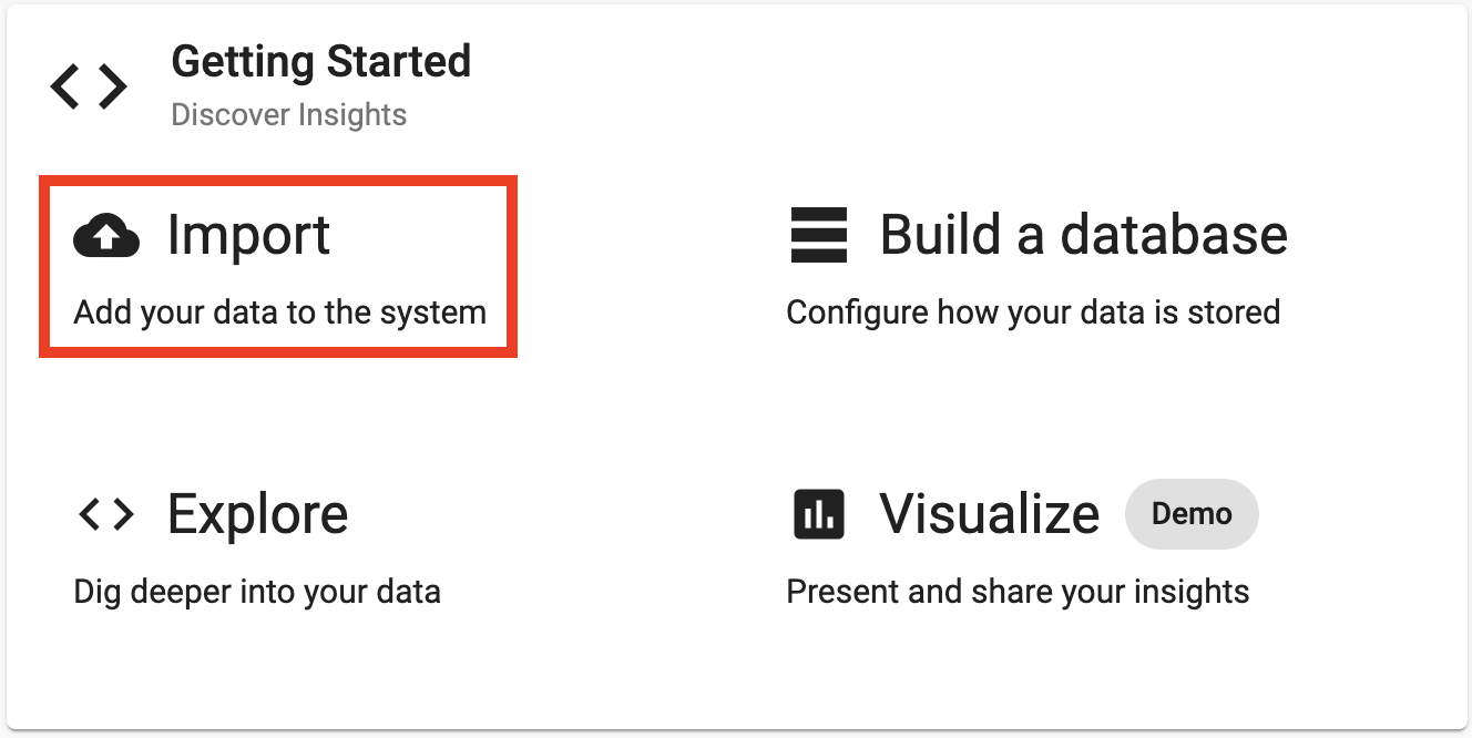
Select Build a database from the home screen Getting Started page.
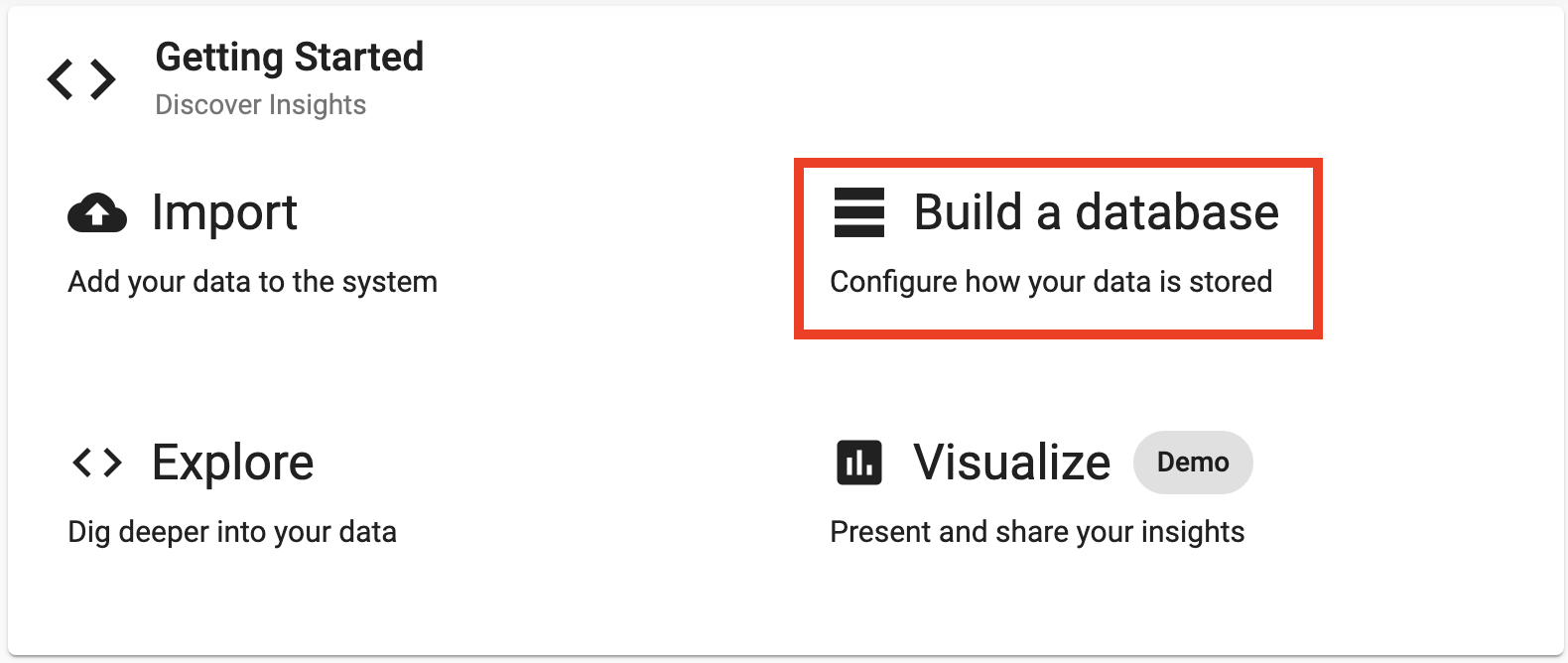
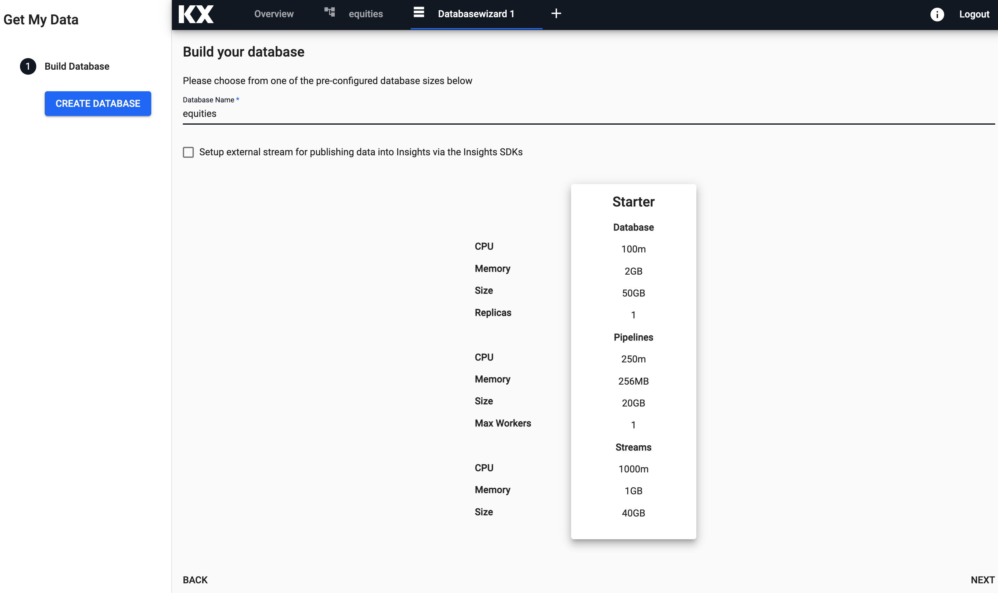
From here, you can enter the name and select the size of your database. Let's give this database a name and select Next.
Configure Schema
The next step requires the user to know information about the incoming data ahead of time:
- column header names
- kdb+ datatypes
Below are the schemas of the data used in this recipe:
For more information on kdb+ data types see here
The name of the tables, column headers and the kdb+ datatypes can be entered in the Configure Schema page.
Before proceeding, check the Advanced Options located at the bottom of the Schema configuration and ensure the following settings are applied.
For this example table trade we are going to ensure the following settings are configured. If you are configuring a different dataset you can adjust as appropriate.
| setting | value |
|---|---|
| Type | partitioned |
| Partition Column | time |
| Timestamp Column | time |
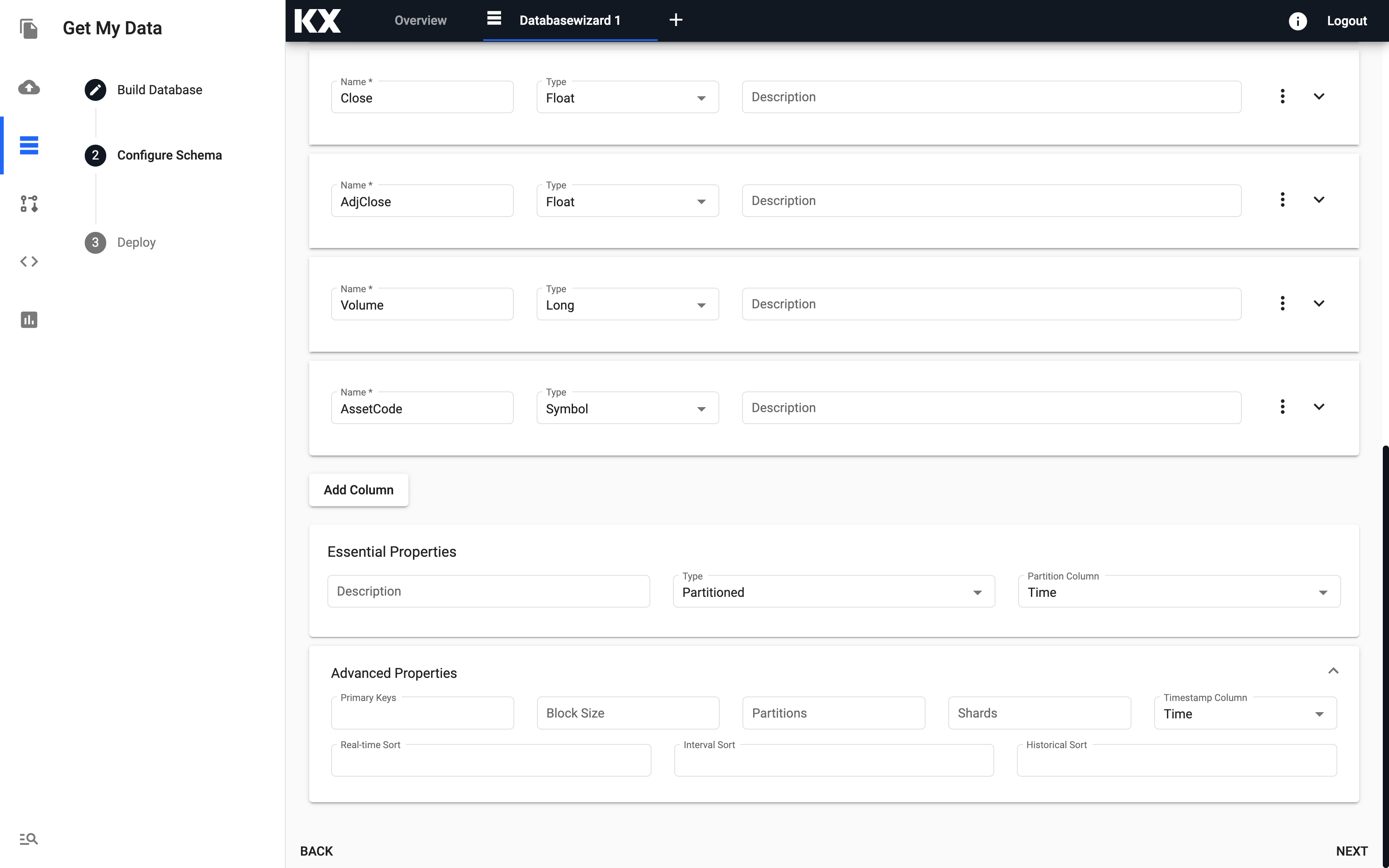
Once all tables have been added, select Next.
Deploy Database
From the next screen you can simply select Save & Deploy.
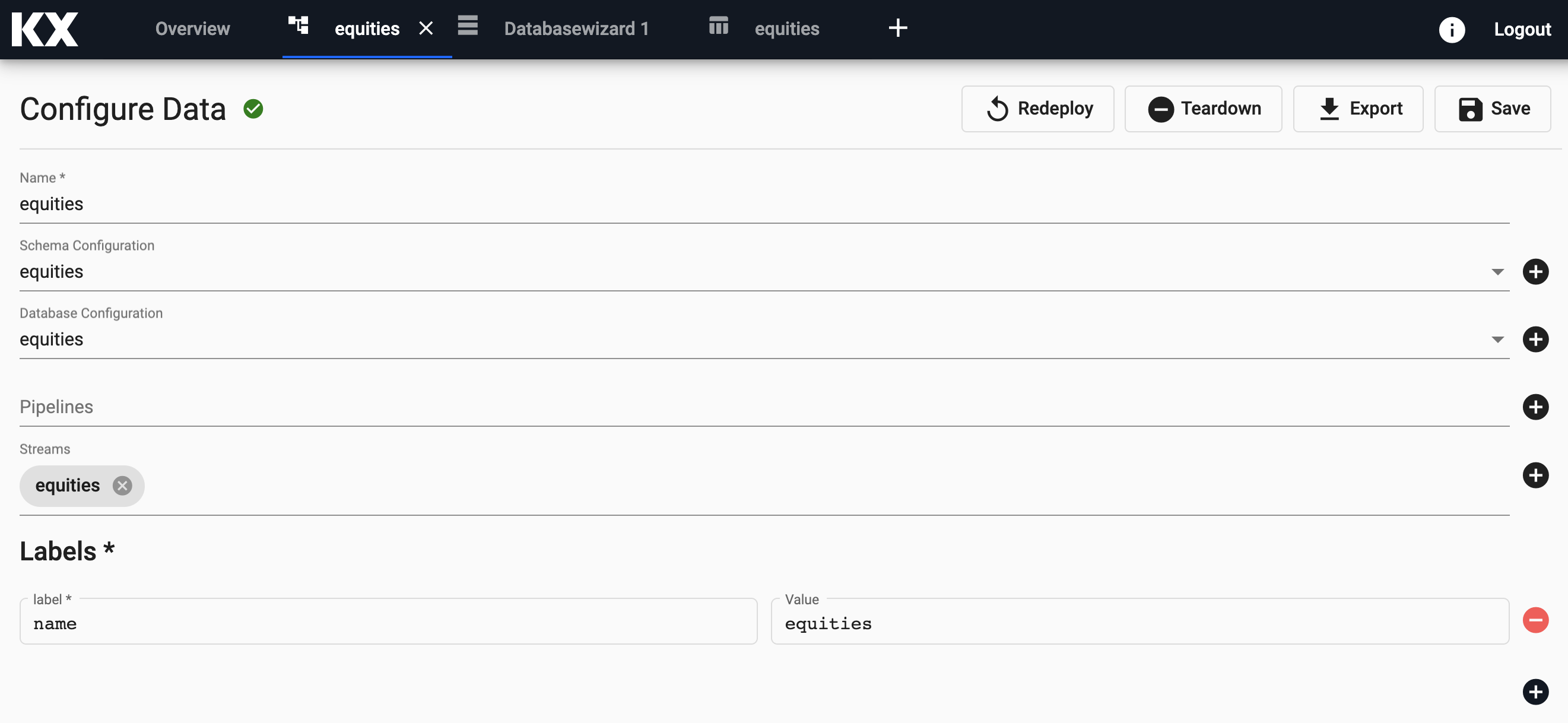
This will take a few seconds and the grey circle will become a green tick and change to Active status when ready.
That's it, you are now ready to Ingest Data!
Step 2: Ingesting Live Data
Importing from Kafka
Apache Kafka is an event streaming platform that can be easily published to and consumed by the KX Insights Platform. The provided Kafka feed has live price alerts that we will consume in this Recipe.
Select Import from the Overview panel to start the process of loading in new data.
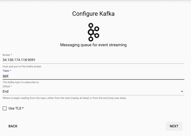
 Select the Kafka node and enter the details as listed below to connect to the datasource.
Here are the broker and topic details for the price feed on Kafka.
| Setting | Value |
|---|---|
| Broker* | 34.130.174.118:9091 |
| Topic* | spx |
| Offset* | End |
 Decoding
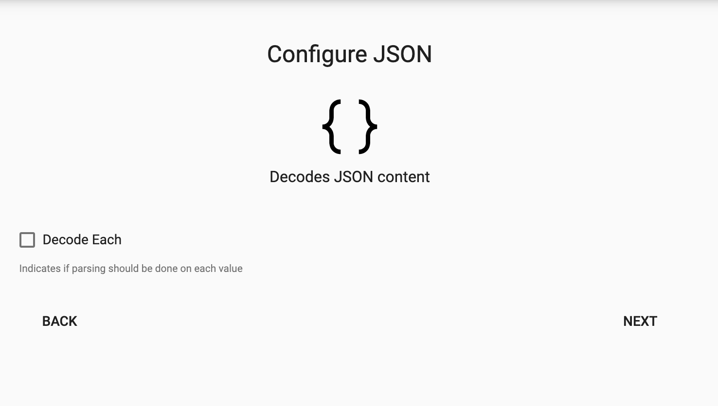
The event data on Kafka is of JSON type so you will need to use the related decoder to transform to a kdb+ friendly format. This will convert the incoming data to a kdb+ dictionary.
Select the JSON Decoder option.
Transforming
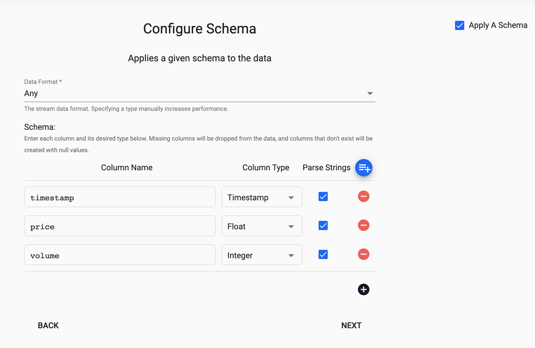
The next screen that comes up is Apply Schema. This is a useful tool that transforms the upstream data to the correct datatype of the destination database.
In the Apply A Schema screen select Data Format = Table from the dropdown.
Next, click on the blue "+" icon next to Parse Strings and you should get a popup window called Load Schema.
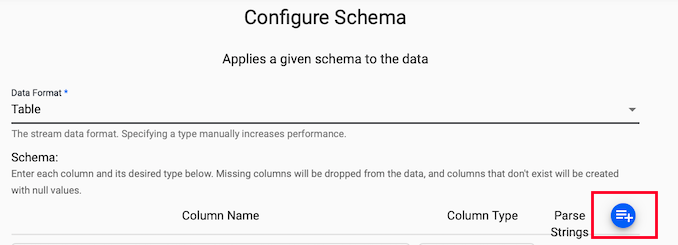
You can then select equities database and trade table from the dropdown and select "Load".
Note, for all fields check the box that says Parse Strings.
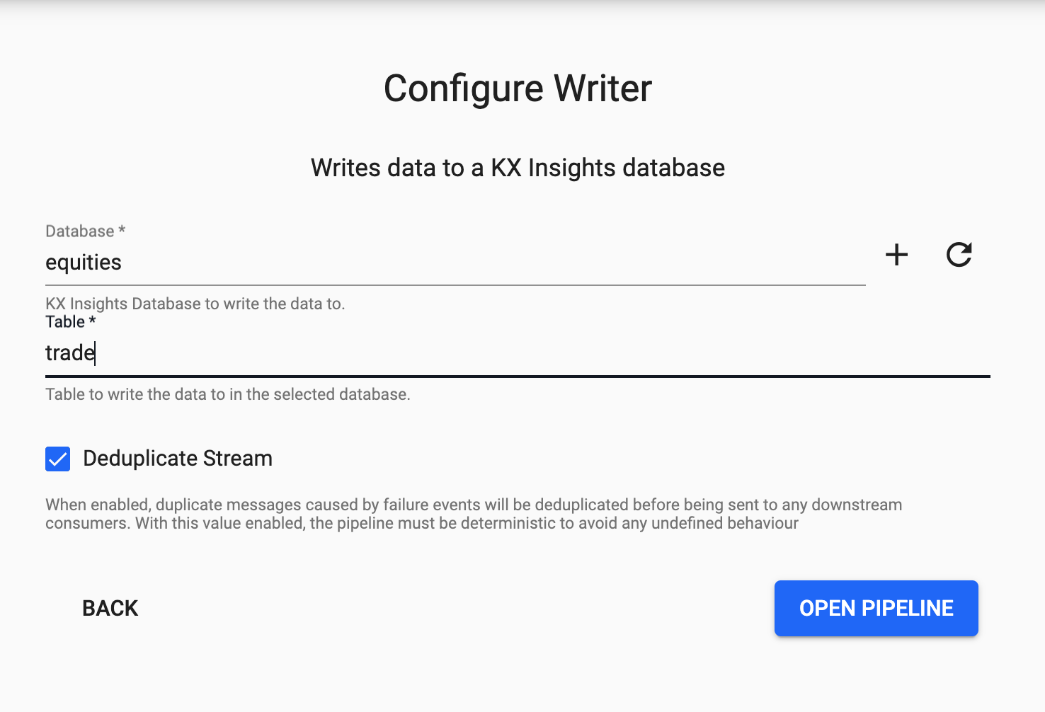
Writing
Finally, from the Writer dropdown select the equities database and the trade table to write this data to and select 'Open Pipeline'.
Apply Function
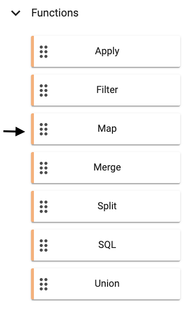
Before we deploy our pipeline there is one more node to add. This data has been converted from incoming JSON format on the Kafka feed to a kdb+ friendly dictionary.
We need to further convert this to a kdb+ table before we deploy so it is ready to save to our database. We can do this by adding a Function node Map. The transformation from the kdb+ dictionary format to kdb+ table is doing using enlist. Copy and paste the below code into your Map node and select Apply.
Additional Functions
For readability additional nodes can be added to continue transforming the data, and moreover, if functions are predefined the name of the function can be provided here to improve reusability.
In this section you are transforming the kdb+ dictionary format using enlist. Copy and paste the below code into your Map node and select Apply.
{[data]
    enlist data
}
You will need to Remove Edge by hovering over the connecting line between the Decoder and Transform nodes and right clicking. You can then add in links to the Function map node.
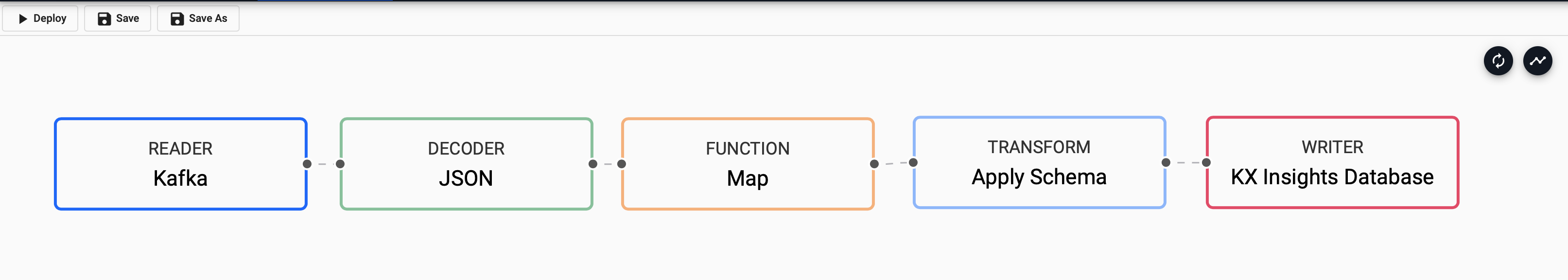
Deploying
Next you can Save your pipeline giving it a name that is indicative of what you are trying to do. Then you can select Deploy.
Once deployed you can check on the progress of your pipeline back in the Overview pane where you started. When it reaches Status=Running then it is done and your data is loaded.
Exploring
Select Explore from the Overview panel to start the process of exploring your loaded data.
Select SQL on the top of the page, you can enter the following SQL to retrieve the count of the trade table.
SELECT COUNT(*) FROM tradeAs new messages appear on the Kafka topic they will be added to the kdb+ table; a rerun of the query will show an increase in the data count as a result.
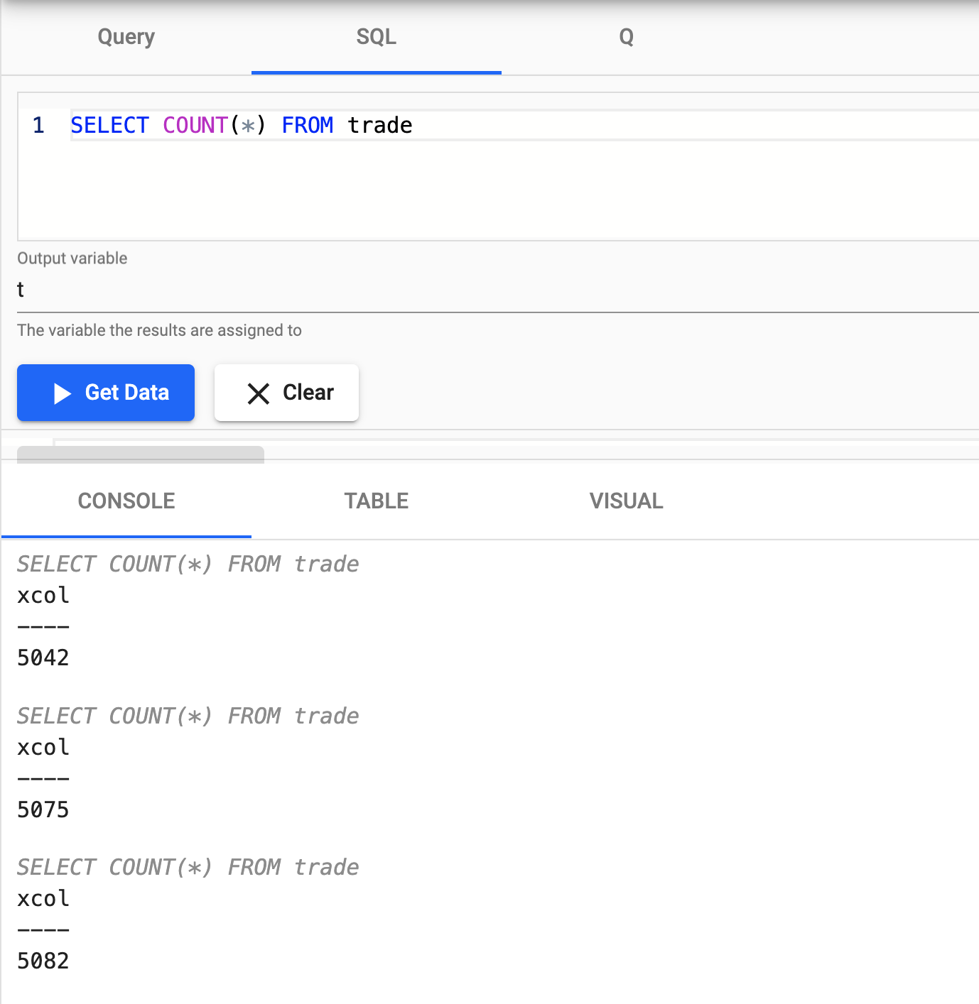
Nice! You have just successfully setup a table consuming live events from a Kafka topic with your data updating in real time.
Step 3: Ingesting Historical Data
Importing from Object Storage
Object storage is a means of storage for unstructured data, eliminating the scaling limitations of traditional file storage. Limitless scale is the reason object storage is the storage of the cloud; Amazon, Google and Microsoft all employ object storage as their primary storage.
In this recipe we will be importing the historical trade data from Azure Blob Storage.
Select Import from the Overview panel to start the process of loading in new data.
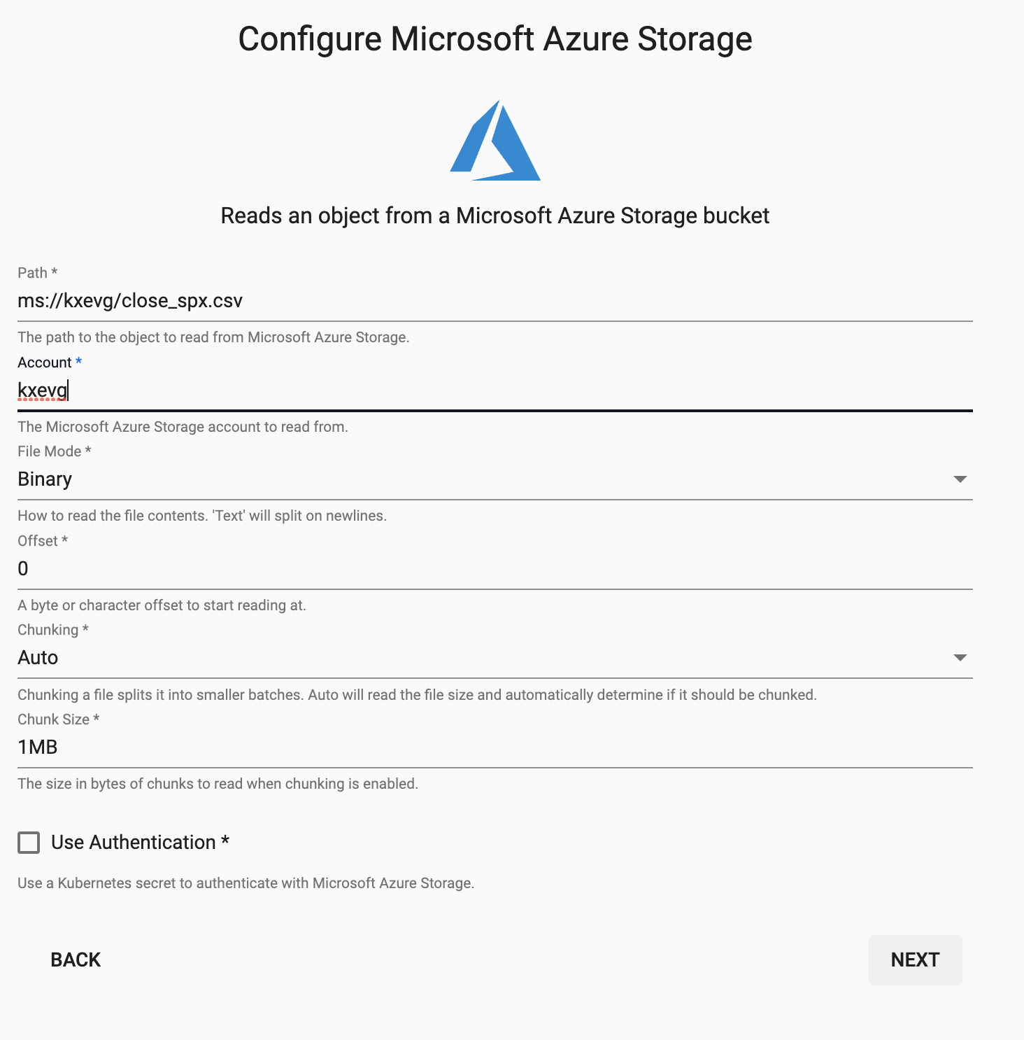
Enter the corresponding details listed to connect to Microsoft Azure Storage.
| setting | value |
|---|---|
| Path* | ms://kxevg/close_spx.csv |
| Account* | kxevg |
| File Mode* | Binary |
| Offset* | 0 |
| Chunking* | Auto |
| Chunk Size* | 1MB |
Decoding
Select the CSV Decoder option.
| setting | value |
|---|---|
| Delimiter | , |
| Header | First Row |
Transforming
The next screen that comes up is Configure Schema. You can select the close table as follow similar steps outlined in the previous section and parse all fields.
Remember to Parse
This indicates whether parsing of input string data into other datatypes is required.Generally for all fields being transformed after being decoded from CSV , select parse.
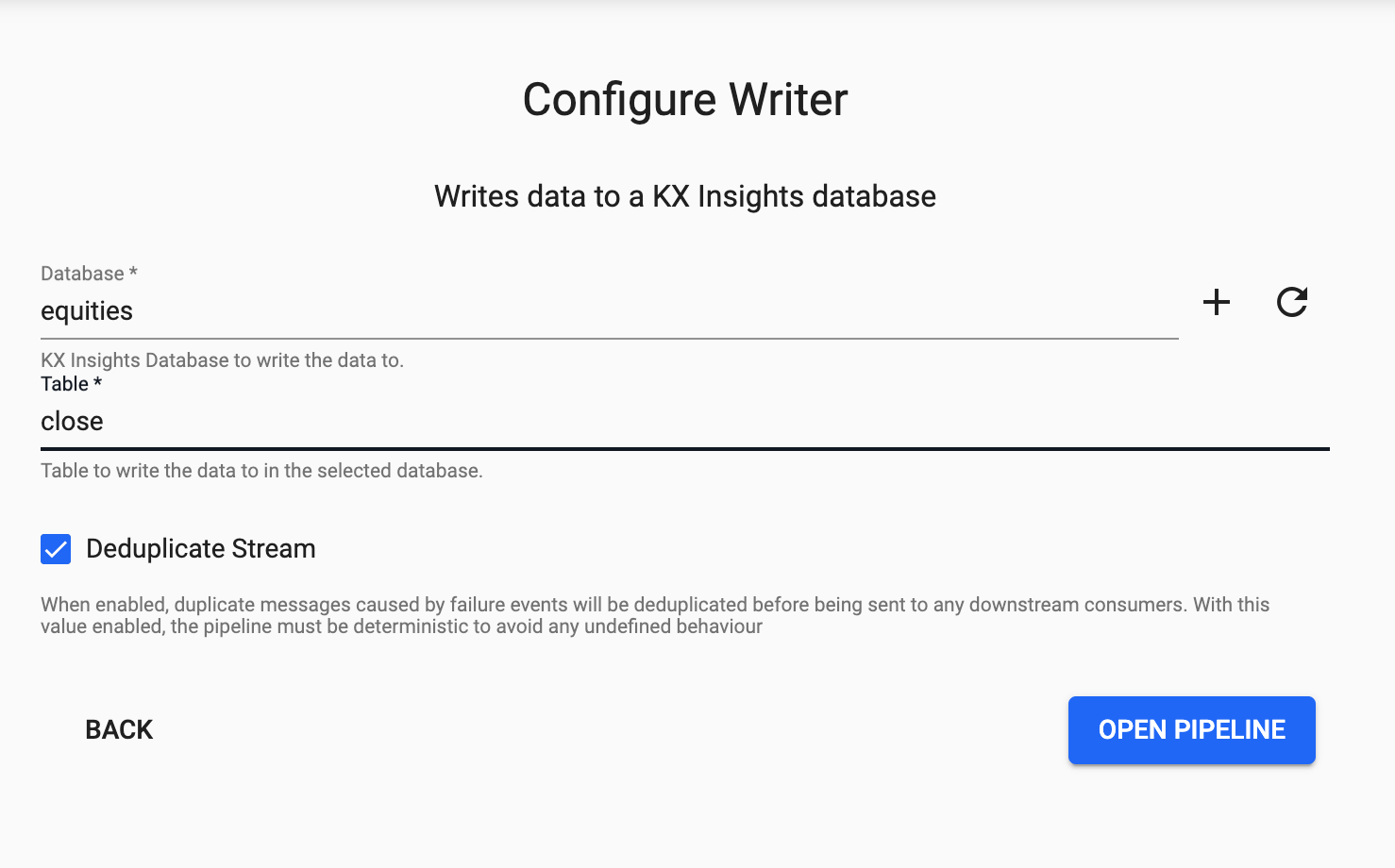
Writing
Finally, from the dropdown select the equities database and the close table to write this data to and select Open Pipeline.
Deploying
The next step is to deploy your pipeline that has been created in the above Importing stage.
You can first Save your pipeline giving it a name that is indicative of what you are trying to do. Then you can select Deploy.
Once deployed you can check on the progress of your pipeline back in the Overview pane where you started. When it reaches Status=Running then it is done and your data is loaded.
Exploring
Select Explore from the Overview panel to start the process of exploring your loaded data.
Select SQL and enter the following SQL to retrieve count of the close table.
SELECT * FROM close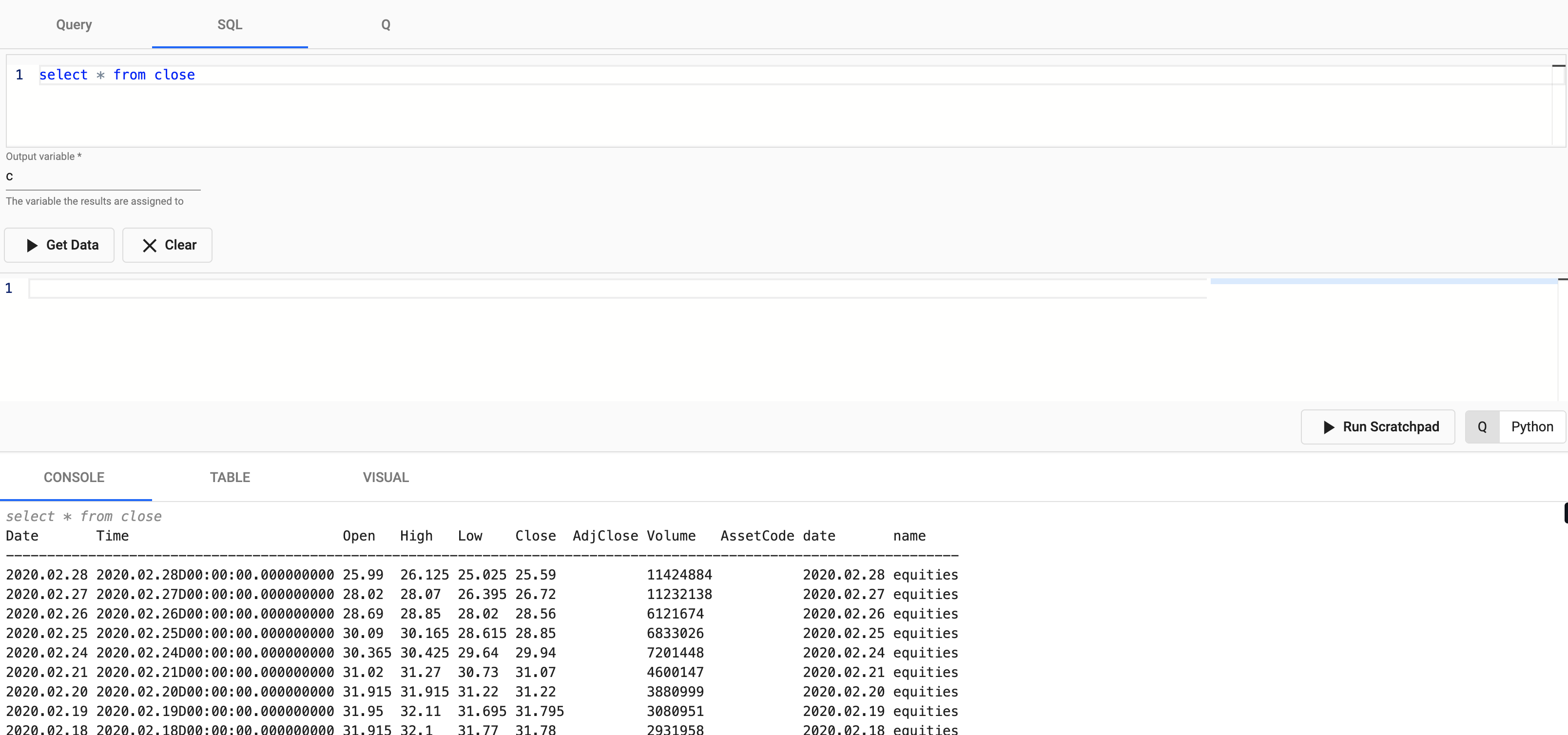
Step 4: Create Powerful Analytics
Prices Over Time
We will query S&P index data to determine the best time to buy and sell. To do this we can run a simple statement:
Select SQL and enter the following SQL to retrieve count of the close table.
SELECT * FROM tradeIn this example, one that displays prices over time.
Long & Short Moving Averages
So far in this recipe, we have just looked at raw data. Where we begin to add real business value is in the ability to run advanced data analytics.
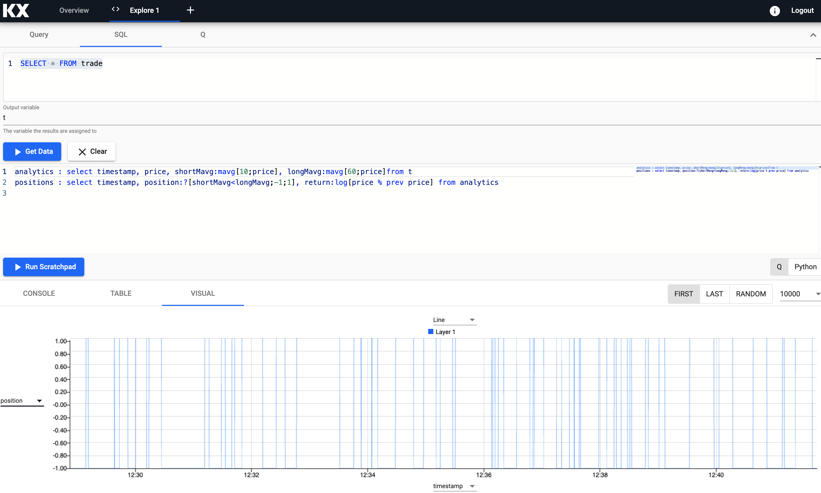
For example, calculating the long and short moving averages of an index, into a variable named analytics and visualising in a new chart.
// taking the close price we calculate two moving averages:
// 1) shortMavg on a window of 10 sec and
// 2) longMavg on a window of 60
analytics : select timestamp,
                   price,
                   shortMavg:mavg[10;price],
                   longMavg:mavg[60;price
            from t
Notice how you can zoom into a particular trading time window for a deeper look at the data trend at a point in time.
Positions
Next, let's create a new variable called positions that uses the data derived from the previous analytics table that will help indicate when to buy and sell our assets.
// when shortMavg and long Mavg cross each other we create the position
// 1) +1 to indicate the signal to buy the asset or
// 2) -1 to indicate the signal to sell the asset
positions : select timestamp,
                   position:?[shortMavg<longMavg;-1;1],
                   return:log[price % prev price]
                from analytics
q/kdb+ functions explained
If any of the above code is new to you don't worry, we have detailed the q functions used above:
- ?[x;y;z] when x is true return y, otherwise return z
- x<y returns true when x is less than y, otherwise return false
- log to return the natual logarithm
- x%y divides x by y
Active vs. Passive Strategy
Active strategy requires someone to actively manage a fund or account, while passive investing involves tracking a major index like the S&P 500 or another preset selection of stocks. Find out more about each, including their pros and cons, on Investopedia.
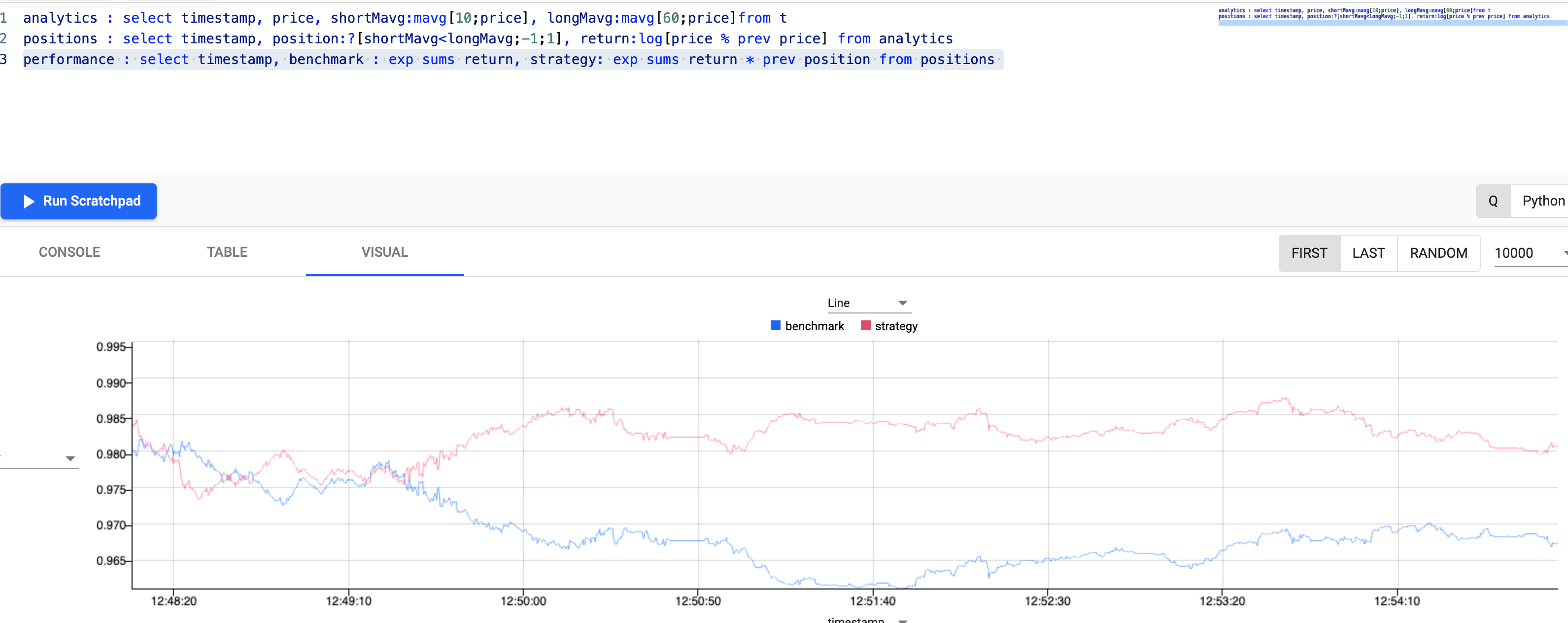
In this recipe we will look to determine if our active strategy performs better than our passive one. To do this we will add new indicators that compare the two and save it a variable called performance.
performance : select timestamp,
                     benchmark: exp sums return,
                     strategy: exp sums return * prev position
                from positions
q/kdb+ functions explained
If any of the above code is new to you don't worry, we have detailed the q functions used above:
- exp raise e to a power where e is the base of natual logarithms
- sums calculates the cumulative sum
- * to multiply
- prev returns the previous item in a list
As you can see in the chart visualization, the active strategy in red outperforms the passive benchmark position in blue, suggesting the potential for greater returns using an active strategy.
Step 5: Reporting
In the previous section we saw that we can create new variables from within the Explore window and visualize on the fly there.
There is also a further reporting suite that can be accessed selecting Reports from the Overview pane. Visualizations can be built using drag-and-drop and point-and-click operations in an easy to use editor.
Reports can only use data that has been persisted to a database
By default Reports can only access data that has been saved to an existing database. So in order to use derived data like the analytics created in the previous section, we must first save the output to a database.
Persisting Analytics
In cases where we want the results of our scratchpad analytics to persist we use a pipeline. Better still, we can do this by simply amending our earlier pipeline from Step 2.
Start by opening the pipeline created in Step 2 - we will be adding some new nodes to it.
Our desired output is to have one table of trade price data, and a second analytics table with our position signals.
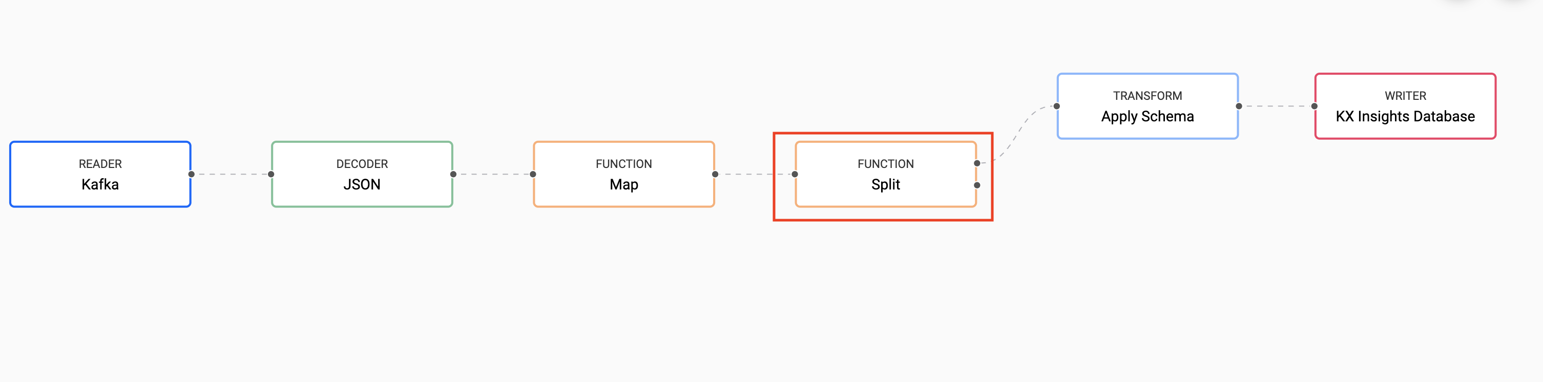
Split Data
The first step is to split the incoming feed. We will do this by adding the Split node just before the schema node in the pipeline.
This node does not require any configuration.
The first branch of the node will continue as before to feed into the Apply Schema node. But details for building our second branch now follow.
This would be a good time to select "Save As" and give your pipeline a new name.
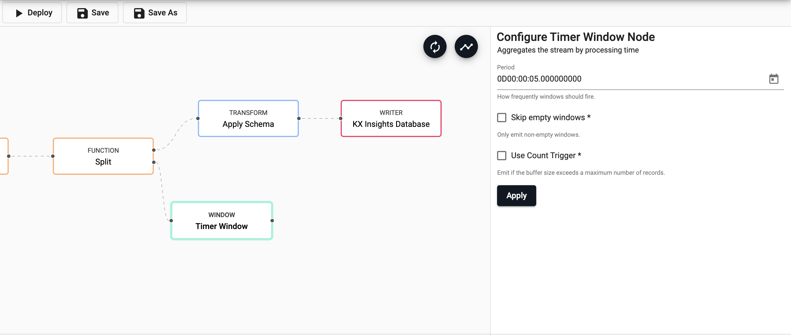
Add Timer Window
Next, we will add a Timer Window node to aggregate the incoming data by time. Data aggregation helps summarize data into a summary form to make it easier to understand and consume by the end user.
We will set the period to be every 5 seconds (0D00:00:05), this will be how often the window should fire.
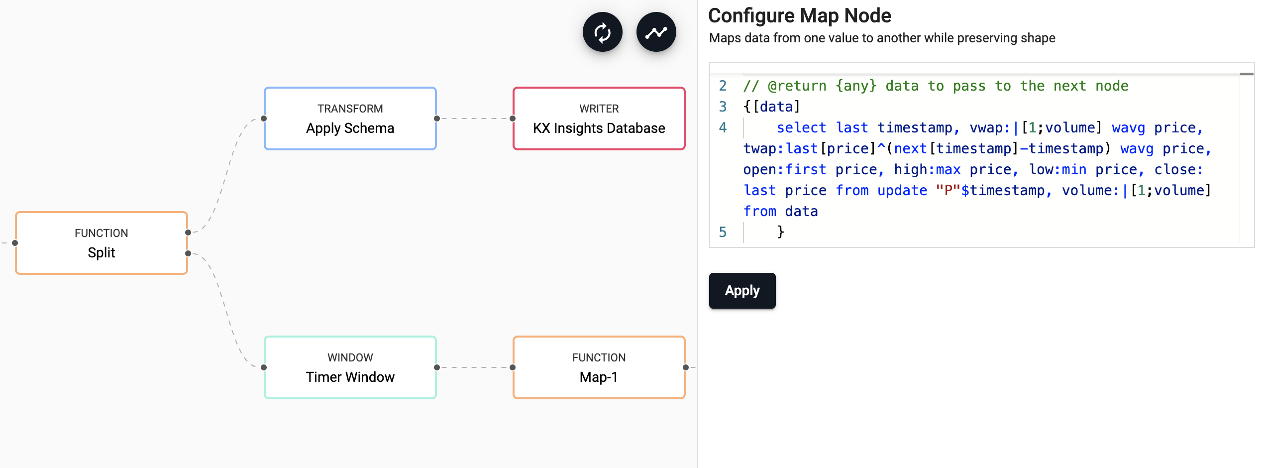
Derivation of Analytics
This is the step in which we add all our business logic that is needed, we will use a Map node here and add the following code:
// the following code is calculating the fields:
// 1) vwap = weighted average price, adjusted by volume, over a given time period
// 2) twap = weighted average price over a given time period
// 3) open = price at which a security first trades when an exchange opens for the day
// 4) high = highest price security is traded at
// 5) low = lowest price security is traded at
// 6) close = price at which a security last trades when an exchange closes for the day
// 7) volume = volume of trades places
{[data]
    select last timestamp,
           vwap:|[1;volume] wavg price,
           twap:last[price]^(next[timestamp]-timestamp) wavg price,
           open:first price,
           high:max price,
           low:min price,
           close: last price
        from update "P"$timestamp,
             volume:|[1;volume]
    from data
    }
kdb+/q functions explained
If any of the above code is new to you don't worry, we have detailed the q functions used above:
- first/last to get first/last record
- | to return the greater number between 1 and
volume - ^ to replace any nulls with the previous price
- wavg to get weighted average
- - to subtract
- max to get maximum value
- min to get minimum value
- $"P" to cast to timestamp datatype
For those that are interested in learning more and getting a quick and a practical introduction to the q language, check out our Introduction to KX Workshop.
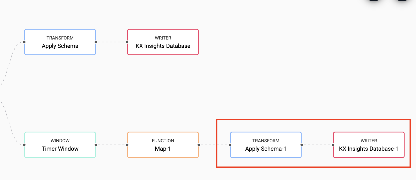
Transform, Write & Deploy
In this final step we will add Transform and Writer nodes, as before to apply our schema and write data down. These steps will be the same as in the previous section.
This time ensure to select to the analytics table in the equities database.
Finally, you can Save your pipeline then you can select Deploy.
Once deployed you can check on the progress of your pipeline back in the Overview pane where you started. When it reaches Status=Running then it is done and your data should be loading in real time to the trade and analytics tables.
Reporting
Now that we have successfully saved down our analytics table we can use the Reports to build some more advanced visualizations.
The Free Trial version of KX Insights Platform comes with a ready-made completed Report called Equities accessible from the left handside toolbar. You can simply open this.
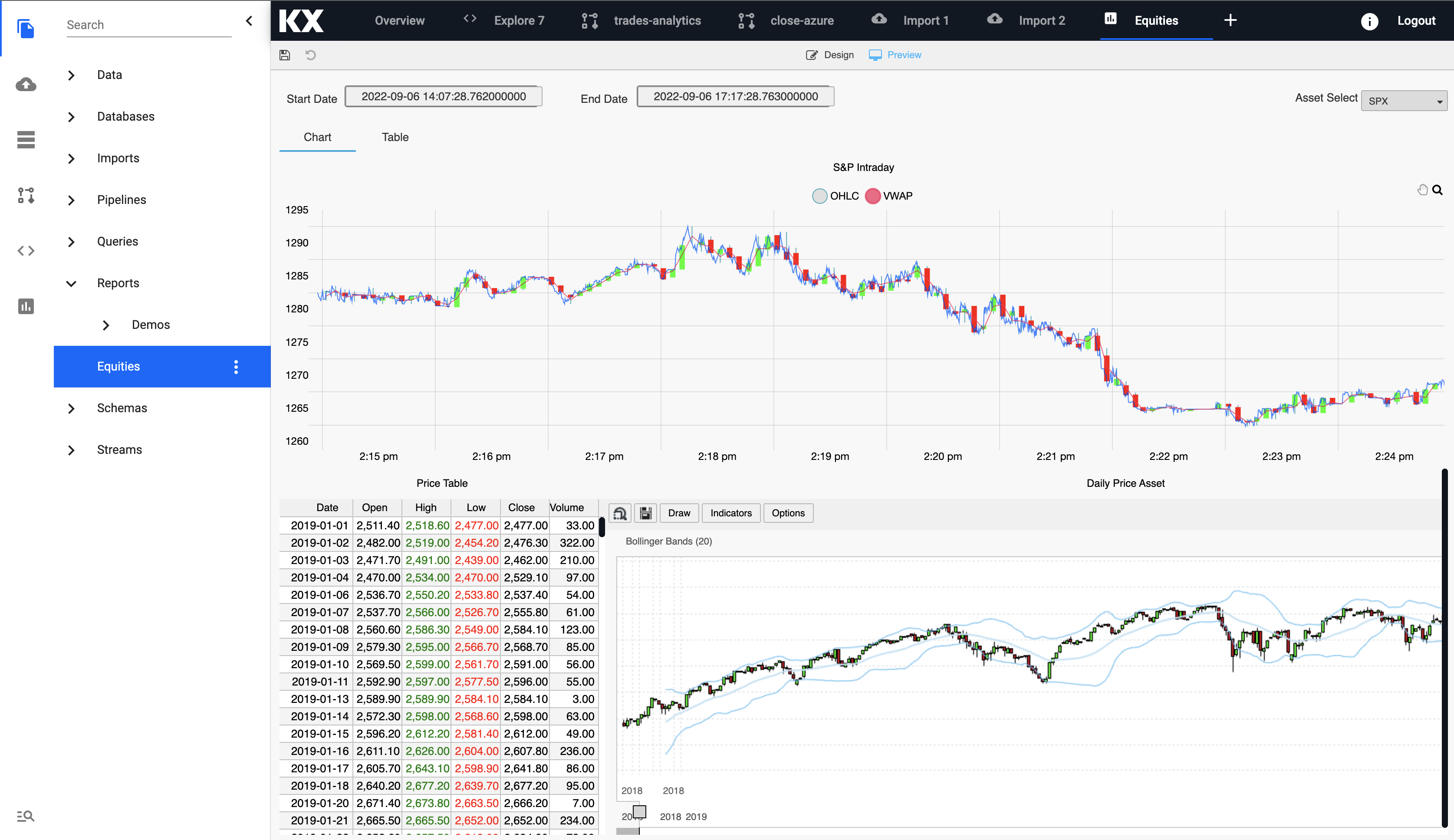
The Equities Report highlights the live Kafka stream and the VWAP, high, low and close data that was derived from the pipelines created earlier in this recipe.
The report also includes daily historical data loaded from our Azure Blob Storage meaning we have both streaming live tick data alongside historical data for the big picture view of the market.
Create your own Report
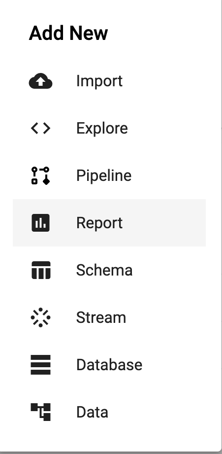
Note, that you can also create your own new Report by selecting the plus icon at the top toolbar and select Report.
Please see our documentation for guidelines on Report creation and design.
You can also download the completed report Equities.json and drop it into a new blank Report.