Grammar of Graphics in q
The documentation here serves as a brief introduction to the scripted visualization library for kdb+ called GG.
For much more detailed information, refer to the .qp and .gg
API references.
The .qp and .gg module families provide data visualization capabilities. The public interface
provides a grammar for specifying how plots should appear, based largely on the idea of mapping
data variables (columns) to positional and aesthetic properties (i.e. x='City',
y='Population', fill='Year'). In general, .qp defines the set of verbs, and .gg the objects.
A basic specification consists of a layer or geometry. A layer is a single set of mappings from variables to properties, together with some data and visual objects. All geometry functions take their positional properties as arguments, and aesthetic properties as optional settings:
.qp.go[500; 500] .qp.scatter[table; `col1; `col2]    // <- table and positional properties
    .qp.s.aes[`fill; `col3]                          // <- aethetic fill property
More advanced specifications can be created by stacking individual layer specifications to create a single new specification. When displayed, the stack of layers will all be rendered onto the same set of axes in the same coordinate system.
Building upon the expressiveness of the Grammar of Graphics, verbs have been added to the grammar for specifying the arrangement of disjoint specifications in order to create a new arranged specification. Any number of specifications can be arranged vertically or horizontally to create new specifications. These new specifications can also be arranged. The only limitation is that arrangements cannot be used within a stack, but a stack can appear in any arrangement. Note, stacks can be stacked themselves.
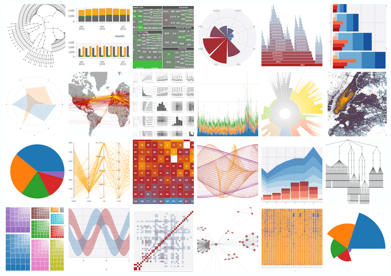
Basic visualization
The most basic way to visualize data is to use the high-level .qp.plot[…] API that takes a table,
a list of columns to plot, and a dictionary of settings (or generic null).
t:([]x:5 * til 45; y: til 45; z: 45?`a`b`c)
// A 500px wide by 500px high plot of all columns of t
.qp.go[500;500] .qp.plot[t; (); ::]
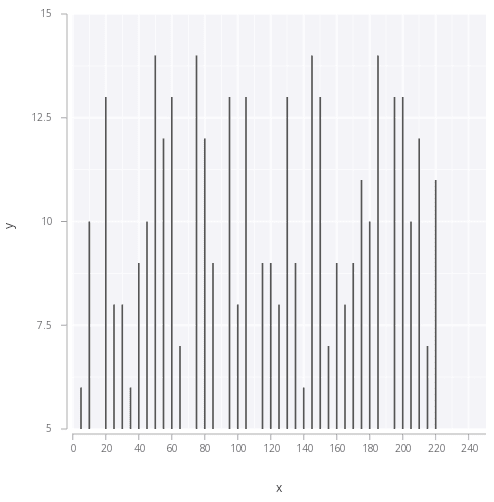
// A plot of only column x
.qp.go[500;500] .qp.plot[t; `x; ::]
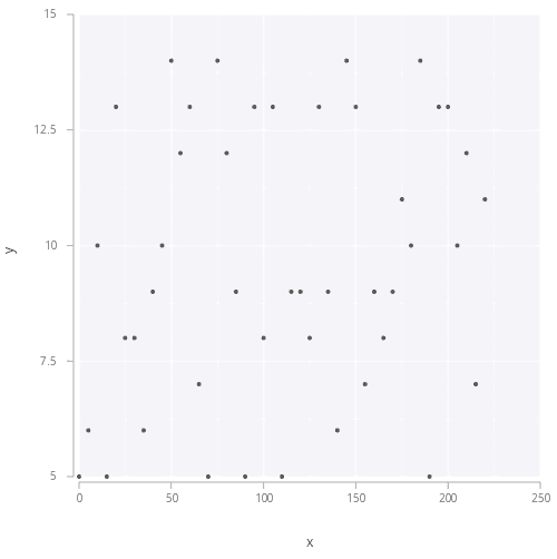
// A plot of x by y
.qp.go[500;500] .qp.plot[t; `x`y; ::]
// A plot of x, y, AND z
.qp.go[500;500] .qp.plot[t; `x`y`z; ::]
In these examples, the .qp.plot[…] section creates a specification – a plot description. The
specification is provided to .qp.go[width; height; spec], which actually renders the plot
description and sends it to the IDE environment. Here are a few example code snippets and
their respective plots:
In the example below, we create a bar using this code:
t:([] x:5 * til 45; y: 45?til 10; z: 45?`a`b`c)
.qp.go[500;500] .qp.bar[t;`x;`y; ::]
In the example below, we create a point or scatter using this code:
t:([] x:5 * til 45; y: 45?til 10; z: 45?`a`b`c)
.qp.go[500;500] .qp.point[t;`x;`y; ::]
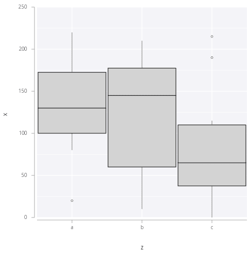
In the example below, we create a boxplot using this code:
t:([] x:5 * til 45; y: 45?til 10; z: 45?`a`b`c)
.qp.go[500;500] .qp.boxplot[t;`z;`x; ::]
This is not the only way to create plot specifications. Very customized plots
can be described by using the Grammar of Graphics rather than the
.qp.plot facility.
Plot specification
A plot is created from an arrangement of stacks of layers.
Layers
At the most basic level, a single layer can be a plot. A layer is a collection of the following properties:
- Data
- Statistical transform (optional)
- Geometry
- Aesthetic mappings
- Scales
- Coordinate system
The data is the table we want to visualize. A statistical transform can be run on the data before visualization to transform the data in any specified way (the default transform is the identity, applying no transformation).
The geometry is the visual mark that will be made for each data record.
There are a number of geometries available (Creating a
layer), such as point, line, rect, etc.
A set of aesthetic mappings map variables from the result of the
statistical transform to attributes of the plot. Each geometry has a set
of required mappings and a set of optional mappings. For example, a
point geometry requires x and y positions to be specified.
Optionally, when using a point, the fill colour, the stroke
colour, the alpha, and the size can also be mapped.
t:([]price:1 2 3; volume:9 8 7; sym:`a`b`c)
For example, if t above is the data for a layer, a possible aesthetic
mapping using a point geometry could be (x='price', y='volume',
fill='sym').
The scales govern the mapping between data variables and aesthetic
properties. There are positional and aesthetic scales, for
positional and aesthetic properties respectively. Positional properties
can have scales such as linear, log, power, etc. Aesthetic scales
can be gradient, circle radius, line size, etc.
Finally, a coordinate system for the mapping to occur in must be present in the layer as well. By default, the coordinate system is assumed to be Rectangular.
Creating a layer
In .qp, each geometry is a function. See the
geometries API references for
more information.
The first argument is the data to be
visualized. The following arguments change based on the geometry, and
are the positional columns for the given geometry. For example, a point
geometry requires an x and y
position, so the signature for creating a layer with a point geometry
is:
.qp.point[t; `price; `volume; ::]
That last argument is a slot for options and customizations. Passing in
generic null (::) will create a basic layer. Every geometry has this same
last argument.
Customizing a layer
The basic plot can be customized by joining options in place of the
last argument. The options are all in the .qp.s sub-namespace. For
example, to add a new fill mapping with an associated scale:
.qp.point[t; `price; `volume]
    .qp.s.aes   [`fill; `sym]
  , .qp.s.scale [`fill; .gg.scale.colour.cat10]
The generic null is omitted, and a list of joined options are passed
instead. The first is a new aesthetic mapping using .qp.s.aes[…],
which takes the aesthetic being mapped (fill) as a symbol, followed by a
column name. This is joined with a new scale governing the fill
aesthetic mapping, using .qp.s.scale[…]. The scale provided here
.gg.scale.colour.cat10 is one of the options for categorical color
scales. It defines 10 distinct colors to map to distinct symbols in the
data. Other options can be added by joining them in the same way.
There are a number of settings available. Refer to the layer settings API reference for more information.
Stacking layers
Multiple layers can be stacked together to create more interesting plots. For example, if there are two tables to visualize:
tableA : ([]a: 1 2 3; b: 4 5 6)
tableB : ([]a: 9 8 7; b: 6 5 4)
and a layer for each table:
.qp.point[tableA; `a; `b; ::]
.qp.line[tableB; `a; `b; ::]
both layers could be rendered on the same axes by stacking with
.qp.stack (…):
.qp.stack (
    .qp.point[tableA; `a; `b; ::];
    .qp.line[tableB; `a; `b; ::]
)
The positional (X and Y) scales and the coordinate system of the first layer in the stack will be inherited by all other layers. For example, if both layers in the above stack should be plotted in a log-log polar plot, it is sufficient to update only the first specification:
.qp.stack (
    .qp.point[tableA; `a; `b]
        .qp.s.scale [`x; .gg.scale.log]
      , .qp.s.scale [`y; .gg.scale.log]
      , .qp.s.coord [.gg.coords.polar];
    .qp.line[tableB; `a; `b; ::]
)
These stacks can be used to create data-specific visualization, such as the following depiction of flights, which is a stack of polygon, segment, and point geometries:
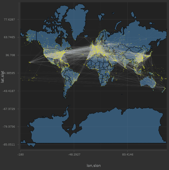
The specification for the above depiction of airports and flights would be:
.qp.stack (
    .qp.polygon[world; `lon; `lat; ::];
    .qp.point[airports; `lon; `lat; ::];
    .qp.segment[flights; `slon; `slat; `dlon; `dlat; ::]
)
This plot also makes use of one of the pre-built color themes, e.g. .gg.theme.dark. See the
section below regarding themes.
Arranging layers
Once multiple plots have been constructed, it is possible to arrange the individual plots in a single visual display. Both of the plots above could be laid out horizontally with:
.qp.horizontal (
    .qp.point[tableA; `a; `b; ::];
    .qp.line[tableB; `a; `b; ::]
)
or vertically with:
.qp.vertical (
    .qp.point[tableA; `a; `b; ::];
    .qp.line[tableB; `a; `b; ::]
)
Arrangements can be arranged as well, so more complicated arrangements can be constructed by layering the arrangements:
.qp.vertical (
    .qp.point[tableA; `a; `b; ::];
    .qp.horizontal (
        .qp.line[tableB; `a; `b; ::];
        .qp.path[tableB; `a; `b; ::]
    )
)
Arrangements can be used to create effective summaries of data. Coupled with dependency specifications, arrangements can also be very effective in data exploration.
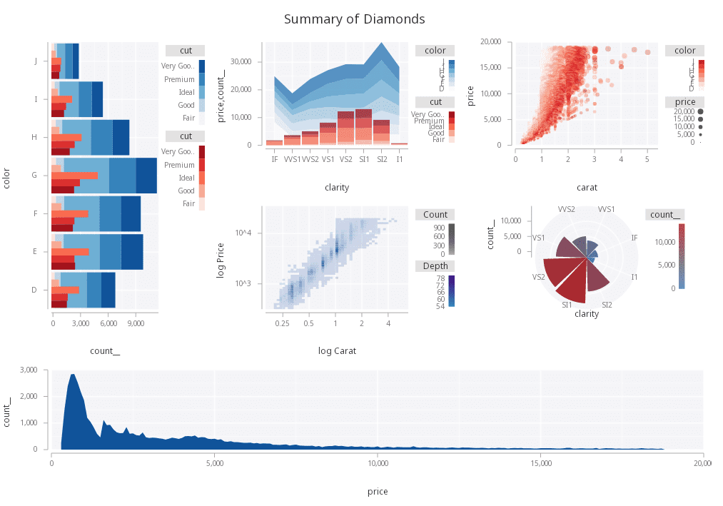 Summary of all data along multiple columns
Interaction
The images produced are interactive. Points can be interrogated by clicking the image. A table of matching records will appear under the image. One such table will appear for every layer in the plot clicked. (Independently-arranged visuals do not contribute).
A plot can also be zoomed by pressing Ctrl+Click (Windows and Linux) or ⌘Click (macOS) and dragging a region within the image in a single plot. The first point must be within the plot axes. The two points of the drag (start and end) define the region to zoom into. After releasing the mouse button, a new image will be drawn and will appear as a new tab.
Specifying dependencies
Two sorts of dependencies exist within .qp. The first is between
layers in independent frames within an arrangement. Consider the
following specification:
t : ([]x:5 * til 45; y: til 45; z: 45?`a`b`c);

.qp.vertical (
    .qp.point[t; `x; `y]
        .qp.s.link[`myid];
    .qp.line[t; `z; `x]
        .qp.s.link[`myid])
In the above, there are two layers which would render beside each other
horizontally. Both layers link the same identifier (myid). Because of
this, whenever one of the layers is drilled into, the other linked
layers will render the same subset of the data as the layer that was
interrogated.
The other concept of a dependency exists within a single frame. This concept is useful when a stack of several layers exists where one or more of the layers are really a function of another layer, as is the case between a scatterplot and a scatterplot smooth (a line drawn through the scatterplot). This is depicted in the in the following:
.qp.stack (
    .qp.point[t; `x; `y]
        .qp.s.primary[`myid];
    .qp.smooth[t; `x; `y; ::]
        .qp.s.secondary[`myid])
In this example, the scatterplot smooth is a secondary layer, and the scatter is a primary layer. Since these use the same identifier, whenever the frame is drilled into, only the scatter will be drilled into, and the smooth will be given the drilled scatter data so that it is always in sync.