Transformed TSS
This page explains the Transformed TSS feature in KDB.AI.
If you're already familiar with this topic, you can skip ahead to the How-to perform a Transformed TSS search guide.
Temporal Similarity Search (Transformed TSS) is a method that reduces the overhead of storing time series vectors inside KDB.AI indexes. For example usage, see our GitHub.
The key components to understand are:
- Time series data
- The performance impact of Window only
- How Transformed TSS reduces memory
- How Transformed TSS manages non-uniform size windows,
- Which data classification is most suited to Transformed-TSS
- Best practices
Time series data
Vector databases can optimise the return of the nearest neighbors of a query vector for fast retrieval and high recall. Indexes do a lot of pre-work, allowing extremely fast retrieval compared to traditional brute-force methods. However, when exploring timeseries data, there are a lot of very big vectors, for example, thousands of points in a 10-minute rolling window and many records. This highlights how memory intensive vector databases can be.
A common use is Retrieval Augmented Generation (RAG) workflows, where vectors are derived from textual sources, and a close proximity of these vectors implies semantic similarity in the underlying text.
Sliding windows of time series data is another collection of vectors (see this example on our website). In this case, the nearest neighbors are the windows of time series data with the highest similarity to a query window. This facilitates time series similarity searches that leverage the performance of KDB.AI to identify nearest neighbors. A straightforward way to construct these vectors would be to aggregate a Sliding window of size D on a time series column, then store the vectors in KDB.AI. This approach has a few drawbacks due to the scaling of data with window size.
Performance impact of Window only
- Memory Overhead: At query time, KDB.AI demands a large amount of memory to return the nearest neighbors due to the high dimensionality (D) of the sliding windows.
- Disk Space: Saving the vectors to disk requires approximately D times the size of the time series column of disk space when using a step size of one between windows.
- Insertion/Query Times: The insertion and retrieval times of longer vectors compared to the same number of shorter vectors is slower.
Additionally, windowing by fixed points can be limiting. It may be more applicable to window temporally, which does not necessarily imply a consistent number of points between windows.
Reducing memory using Transformed TSS with KDB.AI
KDB.AI offers a method to reduce memory and disk overhead when storing time series vectors, with faster retrieval times compared to a Window only approach. This is a small sacrifice to the recall and precision achieved by inserting the raw windows.
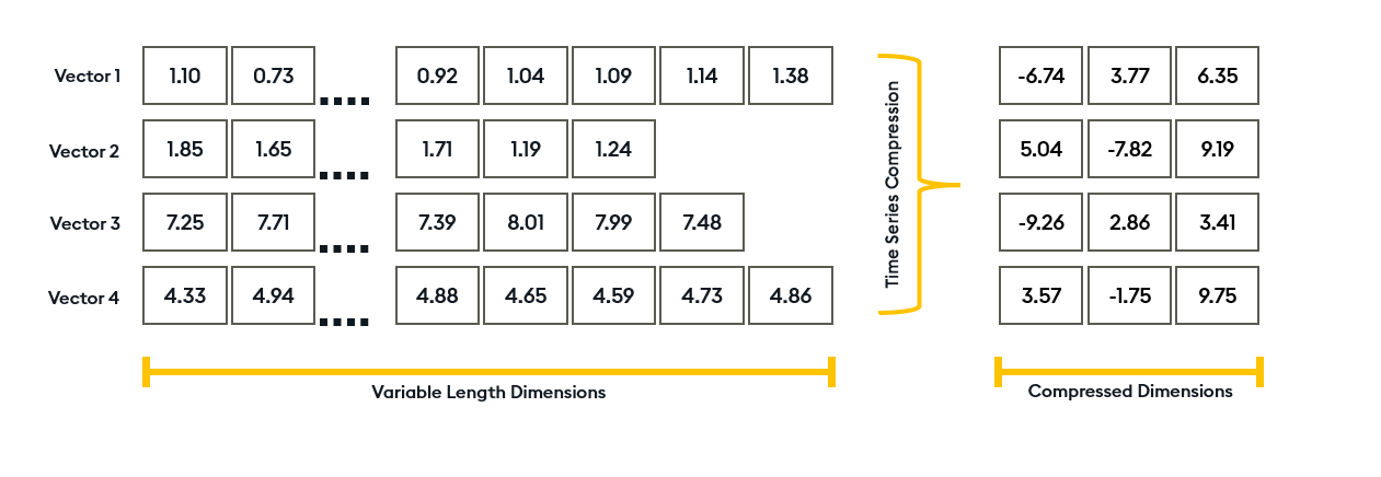
The method dimensionally reduces time series vectors in a way that preserves the majority of the similarity between vectors. This helps you utilize the power of vector databases at scale. See the following visual representation of dimensionality reduction:

Transformed TSS dimensionally reduces your timeseries windows to a point that makes it feasible to utilise vector databases by cutting dimensionality between 8-12, while still getting a high recall. Compared to RAW window insertion this can be 500x smaller vectors, which leads to memory, disk, and query speed improvements (can be 10x compared to RAW windows).
Non-uniform window sizes
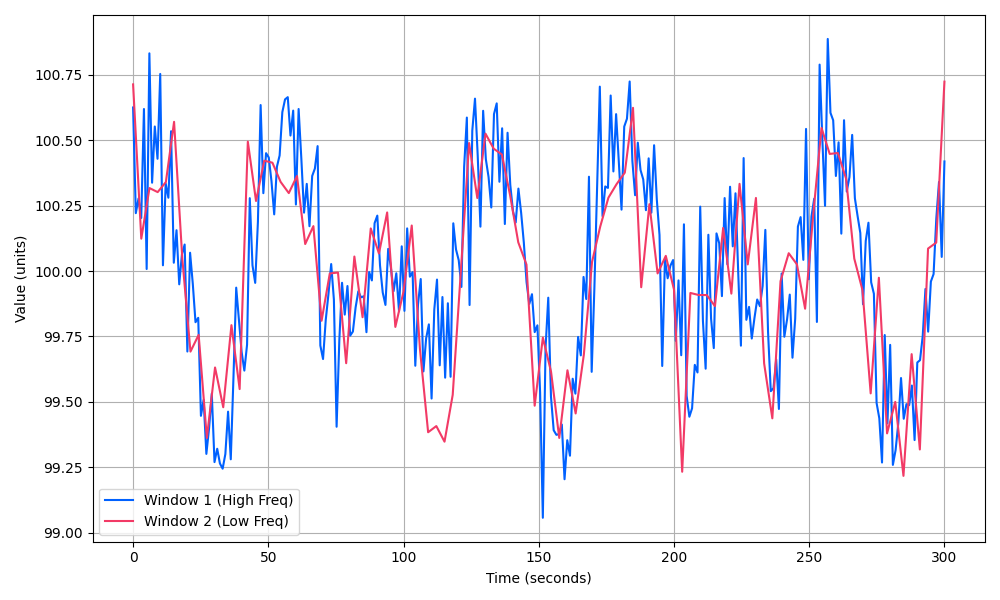
The application of Transformed TSS forces windows to conform to a fixed dimensionality for storage within the index. This means input vectors of differing lengths are considered equally, as you can see below:

The above diagram depicts two series with differing lengths. When considered in the same temporal window, these series display a high level of correlation, however, on a point-by-point basis they do not. This is a typical occurrence in a number of fields, for example, sensors with different sampling rates, or assets with different tick rates due to trading frequency.
Transformed TSS associates the windows to an individual index as if they are mapped to the same domain (similar to the overlay in the above diagram). This provides more control when you construct windows and is useful for enabling fixed-time window searches.
Data classification
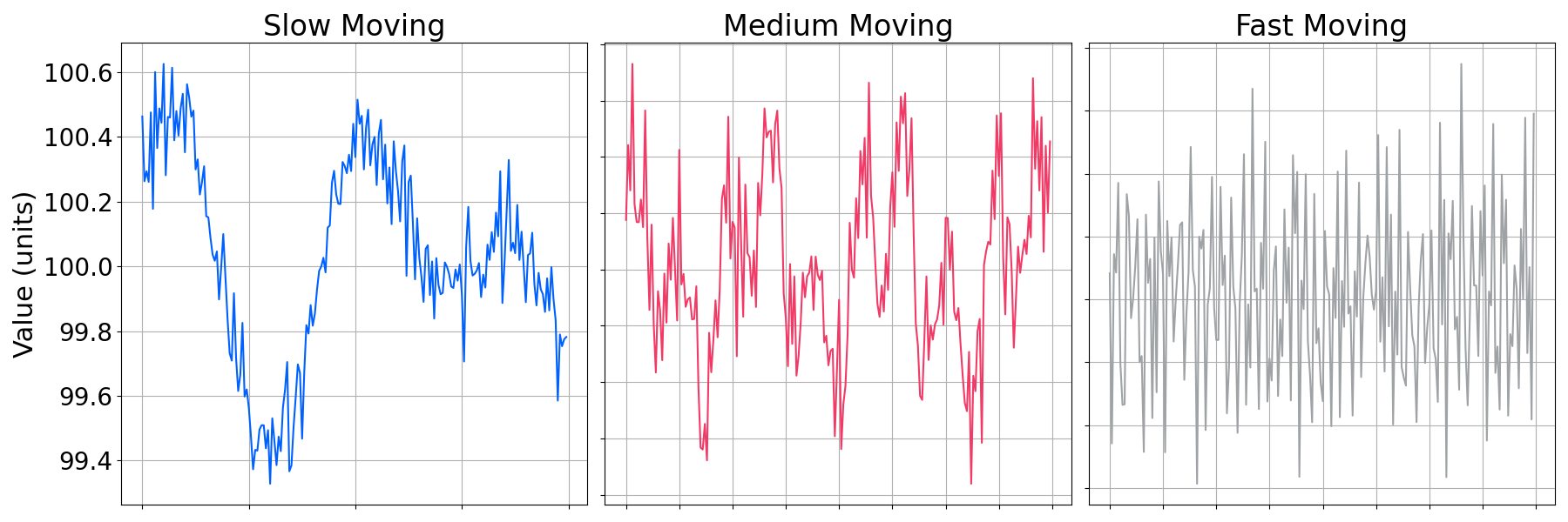
A consequence of dimensionality reduction is that information is inevitably lost. Transformed TSS puts the highest importance on the macroscopic movement and trends of time series patterns. Therefore, it's best to use it for predominantly smooth and continuous data over the windows supplied.

The above diagram shows differing movement levels of data with labels. The rules of thumb for these profiles of data, where dims is the key-value pair defined in the schema for Transformed TSS, are:
| Data classification | Transformed TSS suitability | Suggested dims |
|---|---|---|
| Slow Moving | High | 8 |
| Medium Moving | High | 12 |
| Fast Moving | Low | >20 |
These are recommendations of the value of dims and not fixed.
For Fast moving vectors, use smoothing functions, such as Exponential Moving Average (EMA). You can reduce your window sizes to make the vectors appear less turbulent. If either of these techniques remove significant features of interest from your set of fast moving vectors, it's best to not apply Transformed TSS.
Data cleansing
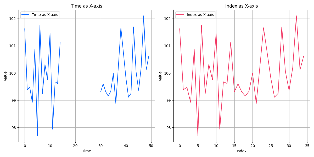
With both Window only and Transformed TSS, vectors are considered one-dimensionally. This impacts how we manage gaps. The below figure on the left shows time series data with a time gap. The figure on the right shows how an index would compare the pattern. It's best to consider this if you're doing fixed point windowing and if windows have differing timesteps within the same window.

To prepare data that contains gaps for insertion into an index, resample windows at a constant frequency or perform interpolation between gaps to impose consistent steps between points of the same vector.
Furthermore, you should apply data cleansing and filtering best practices. You can also use normalisation, depending on the data and how you intend to search for similarities between vectors.
Next steps
Now that you're familiar with the Transformed TSS concepts, try the following:
- Go to the How to perform a Transformed TSS search page and follow the steps.
- Visit the KDB.AI Learning hub for time series insights with Temporal Similarity Search.