1. Q Shock and Awe¶
The purpose of this chapter is to provide a whirlwind tour of some highpoints of q. We don't expect everyone to follow everything the first time through but we do expect that you will be impressed by the power and economy of q. The examples here should motivate careful reading of the following chapters. Once you complete the main text, come back to this chapter and you'll breeze through it.
1.1 Starting q¶
Your installation of q should have placed the q executable in $HOME/q (or $QHOME) on Unix-based systems, or in the q directory on the C: drive on Windows.
For Windows, start a q session by typing q on the command line; for Linux-based systems use rlwrap q so that you will have command line recall. You should see a new q session with the Kx Systems copyright notice followed by the q prompt indicated by a leading q) on the command line. This is the q console. Type 6*7 and press Enter or Return to see the result.
q)6*7
42
q)☐
Here the ☐ represents the cursor awaiting your next input.
Note
In this document, sample q console sessions will always be displayed in fixed-pitch type with shaded background. As a pedagogical device, in many q snippets we suppress the console response to an entered q expression, replacing it with an underscore. This means that you, the serious student, are expected to enter this expression into your own q session and see the result.
q)"c"$0x57656c6c20646f6e6521
_
You did do this, didn’t you? This is a tutorial.
1.2 Variables¶
In q, as in most languages that allow mutable state, a "variable" should properly be called an "assignable". (See Mathematical Refresher above for a discussion). Nevertheless, a variable in q is a name together with associated storage that holds whatever value has been most recently assigned to the variable. As a consolation, at least q does not misuse = for assignment, as do many languages; in q = actually means "test for equality."
Declaring a variable and assigning its value are done in a single step with the operator : which is called amend and is read "is assigned" or "gets." Here is how to create and assign variable a with integer value 42.
q)a:42
q)_
When you entered this in your q session, you noted that nothing is echoed to the console. In order to see that a has indeed been assigned, simply enter the variable.
q)a
42
A variable name must start with an alphabetic character, which can be followed by alpha, numeric or underscore.
Naming Style Recommendations
-
Choose a name long enough to make the purpose of the entity evident, but no longer. The purpose of a name is to communicate to a reader of the code at another time – perhaps even you. Long names may not make code easier to read. For example,
checkDiskis clearer thancdorchkbut is no less clear thancheckDiskForFileConsistency. -
Use verbs for function names; use nouns for data.
-
Be consistent in your use of abbreviations. Be mindful that even "obvious" abbreviations may be opaque to readers whose native language is different than yours.
-
Be consistent in your use of capitalization, such as initial caps, camel casing, etc. Pick a style and stick to it.
-
Use contexts for name spacing functions.
-
Do not use names such as
int,floator other words that have meaning in q. While not reserved, they carry special meaning when used as arguments for certain q operators. -
Accomplished q programmers avoid using the underscore character in q names. If you insist on using underscore in names, do not use it as the last character. Expressions involving the built-in
_operator and names with underscore will be difficult to read.
1.3 Whitespace¶
In general, q permits, but does not require, whitespace around operators, separators, brackets, braces, etc. You could also write the above expression as
a : 42or,
a: 42Accomplished q programmers view whitespace around operators as training wheels on a bicycle.
Because the q gods prefer compact code, you will see programs with no superfluous whitespace… none, zilch, zip, nada. In order to help you get accustomed to this terseness, we use whitespace only in juxtaposition and after semi-colon and comma separators. You should feel free to add whitespace for readability where it is permitted, but be consistent in its use or omission. We will point out where whitespace is required or forbidden.
1.4 The Q Console¶
The q console evaluates a q expression that you enter and echoes the result on the following line. An exception to this is the assignment operation – as noted above – that has a return value, even though the console does not echo it. You may wonder why. This is simply a q console design choice to avoid cluttering the display.
To obtain official console display of any q value, apply the built-in function show to it.
q)show a:42
42
1.5 Comments¶
The forward-slash character / indicates the beginning of a comment. Actually, it instructs the interpreter to ignore everything from it to the end of the line.
At least one whitespace character must separate / intended to begin a comment from any text to the left of it on a line.
In the following example, no definition of c is seen by the interpreter, so an error occurs.
q)b:1+a:42 / nothing here counts c:6*7
q)c
'c
Notice the succinct (ahem) format of q errors: a single vertical quote (called "tick" in q-speak) followed by a terse error message. In this case, the error should be interpreted as "Error: c is not recognized."
The following generates an even more succinct error.
q)a:42/ intended to be a comment
'
Coding Style
The q gods have no need for explanatory error messages or comments since their q code is perfect and self-documenting. Even experienced mortals spend hours poring over cryptic q error messages such as the ones above. Moreover, many mortals eschew comments in misanthropic coding macho. Don’t.
V3.5 introduced debugging and more informative error displays. [Ed.]
1.6 Assignment¶
A variable is not explicitly declared or typed. Instead, its assigned value determines the variable type. In our example, the expression to the right of the assignment is syntactically an integer value, so the name a is associated with a value of type long integer. It is permissible to reassign a variable with a value of different type. Once this is done, the name will reflect the type of its newly assigned value. Much more about types in Chapter 2.
Important
Dynamic typing combined with mutable variables is flexible but also dangerous. You can unintentionally change the type of a variable with a wayward assignment that might crash your program much later. Or you can inadvertently reuse a variable name and wipe out any data in the variable. An undetected typo can result in data being sent to a black hole. Be careful to enter variable names correctly.
Many traditional languages permit only a variable name to the left of an assignment. In q an assignment carries the value being assigned and can be used as part of a larger expression. So we find,
q)1+a:42
43
In the following example, the variable a is not referenced after it is assigned. Instead, the value of the assignment is propagated onward – i.e., to the left.
q)b:1+a:42
q)b
43
1.7 Order of Evaluation¶
The interpreter evaluates the above specification of b from right-to-left (more on this in Chapter 4). If it were verbose, the interpreter might say:
The integer 42 is assigned to a variable named
a, then the result of the assignment, namely 42, is added to the integer 1, then this result is assigned to a variable namedb.
Because the interpreter always evaluates expressions right-to-left, programmers can safely read q expressions left-to-right,
The variable
bgets the value of the integer 1 plus the value assigned to the variablea, which gets the integer 42.
This is exactly as in mathematics where we would read f(g(x)) as "f of g of x" even though g is evaluated first and the result passed into f. We just dispense with the parentheses.
Recommendations on Assignment Style
- The ability to chain evaluation of expressions permits a single line of q code to perform the work of an entire verbose program. In general this is acceptable (even good) q style when not taken to the extreme with extremely long wrapped lines or nested sub expressions.
- Intra-line assignments, as above, can simplify code provided they are few and are referenced only within the line of creation.
- It is not bad form to make one assignment per line, provided you don't end up with one operation per line.
- Wannabe q gods carry terseness to the extreme, which quickly leads to write-only code.
1.8 Data Types 101¶
There are q data types to cover nearly all needs but a few basic types are used most frequently. In q3.0 and above, the basic integer type, called long, is a 64-bit signed integer. If you write a literal integer as in the snippets above, q creates a 64-bit signed integer value.
q)42
_
The basic floating point type in q is called float, often known as a "double" in many languages. This is an 8-byte value conforming to the IEEE floating-point specification.
q)98.6
_
Arithmetic operations on integer and float values are pretty much as expected except for division, which is written as % since / has been preempted for comments (as well as other uses). Sorry, that's just the way it is. Also note that division always results in a float.
q)2+3
5
q)2.2*3.0
6.6
q)4-2
2
q)4%2
2f
Boolean values in q are stored in a single byte and are denoted as the binary values they really are with an explicit type suffix b. One way to generate boolean values is to test for equality.
q)42=40+2
1b
q)42=43
_
The two most useful temporal types are date and timespan; both represent integral counts. Under the covers, a date is the number of days since the millennium, positive for post and negative for pre.
q)2000.01.01 / this is actually 0
_
q)2014.11.19 / this is actually 5436
_
q)1999.12.31 / this is actually -1
_
Similarly, a time value is represented by a timespan, which is a (long) integer count of the number of nanoseconds since midnight. It is denoted as,
q)12:00:00.000000000 / this is noon
_
One interesting and useful feature of q temporal values is that, as integral values under the covers, they naturally participate in arithmetic. For example, to advance a date five days, add 5.
q)2000.01.01+5
_
Or to advance a time by one microsecond (i.e., 1000 nanoseconds) add 1000.
q)12:00:00.000000000+1000
_
Or to verify that temporal values are indeed their underlying values, test for equality.
q)2000.01.01=0
_
q)12:00:00.000000000=12*60*60*1000000000
_
The treatment of textual data in q is a bit complicated in order to provide optimum flexibility and performance. For now, we will focus on symbols, which derive from their namesake in Scheme and are akin to VARCHAR in SQL or strings in other languages. They are not what q calls strings!
Think of symbols as wannabe names: all q names are symbols but not all symbols are names. A symbol is atomic, meaning that it is viewed as an indivisible entity (although we shall see later how to expose the characters inside it).
Symbols are denoted by a leading back-quote (called "back tick" in q-speak) followed by characters. Symbols without embedded blanks or other special characters can be entered literally into the console.
q)`aapl
_
q)`jab
_
q)`thisisareallylongsymbol
_
Since symbols are atoms, any two can be tested for equality.
q)`aapl=`apl
_
1.9 Lists 101¶
The fundamental q data structure is a list, which is an ordered collection of items sequenced from left to right. The notation for a general list encloses items with ( and ) and uses ; as separator. Spaces after the semi-colons are optional but can improve readability.
q)(1; 1.2; `one)
_
A few observations on lists.
- A list can contain items of different type; this usually requires wrapping the values in a variant type in other languages. That being said, it is best to avoid mixed types in lists, as their processing is slower than homogenous lists of atoms.
- Assuming you entered the above snippet, you have noticed that the console echoes the items of a general list one item per line.
- In contrast to most functional languages, lists need not be built up by "cons"-ing one item at a time, although they can be. Nor are they stored as singly-linked lists under the covers.
In the case of a homogenous list of atoms, called a simple list, q adopts a simplified format for both storage and display. The parentheses and semicolons are dropped. For example, a list of underlying numeric type separates its items with a space.
q)(1; 2; 3)
1 2 3
q)(1.2; 2.2; 3.3)
-
q)(2000.01.01; 2000.01.02; 2001.01.03)
-
A simple list of booleans is juxtaposed with no spaces and has a trailing b type indicator.
q)(1b; 0b; 1b)
101b
A simple list of symbols is displayed with no separating spaces.
q)(`one; `two; `three)
`one`two`three
Homogenous lists of atoms can be entered in either general or simplified form. Regardless of how they are created, q recognizes a list of homogenous atoms dynamically and converts it to a simple list.
Next we explore some basic operations to construct and manipulate lists. The most fundamental is til, which takes a non-negative integer n and returns the first n integers starting at 0 (n itself is not included in the result).
q)til 10
0 1 2 3 4 5 6 7 8 9
We obtain the first 10 integers starting at 1 by adding 1 to the previous result. Be mindful that q always evaluates expressions from right to left and that operations work on vectors whenever possible.
q)1+til 10
1 2 3 4 5 6 7 8 9 10
Similarly, we obtain the first 10 even numbers and the first ten odd numbers.
q)2*til 10
_
q)1+2*til 10
_
Finally, we obtain the first 10 even numbers starting at 42.
q)42+2*til 10
_
Another frequently used list primitive is Join , that returns the list obtained by concatenating its right operand to its left operand.
q)1 2 3,4 5
1 2 3 4 5
q)1 2 3,100
_
q)0,1 2 3
_
To extract items from the front or back of a list, use the Take operator #. Positive argument means take from the front, negative from the back.
q)2#til 10
0 1
q)-2#til 10
_
Applying # always results in a list.
In particular, the idiom 0# returns an empty list of the same type as the first item in its argument. Using an atom argument is a succinct way to create a typed empty list of the type of the atom.
q)0#1 2 3
`long$()
q)0#0
`long$()
q)0#`
`symbol$()
Should you extract more items than there are in the list, # restarts at the beginning and continues extracting. It does this until the specified number of items is reached.
q)5#1 2 3
1 2 3 1 2
In particular, if you apply # to an atom, it will continue drawing that single atom until it has the specified number of copies. This is a succinct idiom to replicate an atom to a list of specified length.
q)5#42
42 42 42 42 42
As with atoms, a list can be assigned to a variable.
q)L:10 20 30The items of a list can be accessed via indexing, which uses square brackets and is relative to 0.
q)L[0]
10
q)L[1]
_
q)L[2]
_
1.10 Functions 101¶
All built-in q operators and keywords are functions. The main differences between q’s functions and the ones we mortals can write are:
- The built-ins are written and optimized in one of the underlying languages k or C.
- Binary q functions can be used with infix notation – i.e., as operators – whereas ours must be used in prefix form.
Functions in q correspond to “lambda expressions” or “anonymous functions” in other languages. This means that a function is a first-class value just like a long or float value – i.e., it acquires a name only once it is assigned to a variable.
Conceptually, a q function is a sequence of steps that produces an output result from an input value. Since q is not purely functional, these rules can interact with the world by reaching outside the context of the function. Such actions are called side effects and should be carefully controlled.
Function definition is delimited by matching curly braces { and }. Immediately after the opening brace, the formal parameters are names enclosed in square brackets [ and ] and separated by semi-colons. These parameters presumably appear in the body of the function, which follows the formal parameters and is a succession of expressions sequenced by semi-colons.
Following is a simple function that returns the square of its input. On the next line we assign the same function to the variable sq. The whitespace is optional.
q){[x] x*x}
_
q)sq:{[x] x*x}
_
Here is a function that takes two input values and returns the sum of their squares.
q){[x;y] a:x*x; b:y*y; a+b}
_
q)pyth:{[x;y] a:x*x; b:y*y; a+b}
_
To apply a function to arguments, follow it (or its name, if it has been assigned to a variable) by a list of values enclosed in square brackets and separated by semi-colons. This causes the argument expression to be evaluated first, then the expressions in the body of the function to be evaluated sequentially by substituting each resulting argument for every occurrence of the corresponding formal parameter. Normally the value of the final expression is returned as the output value of the function.
Here are the previous functions applied to arguments.
q){[x] x*x}[5]
25
q)sq[5]
_
q){[x;y] a:x*x; b:y*y; a+b}[3;4]
25
q)pyth[3;4]
_
The variables a and b appearing in the body of the last function above are local – i.e., they are created and exist only for the duration of an application.
It is common in mathematics to use function parameters x, y, or z. If you are content with these names (in the belief that descriptive names provide no useful information to the poor soul reading your code), you can omit their declaration and q will understand that you mean the implicit parameters x, y, and z in that order.
q){x*x}[5]
25
q){a:x*x; b:y*y; a+b}[3;4]
25
This is about as pithy as it gets for function definition and application. Well, not quite. In q, as in most functional languages, we don't need no stinkin’ brackets for application of a unary function – i.e., with one parameter. Simply separate the function from its argument by whitespace. This is called function prefix syntax.
q){x*x} 5
_
q)f:{x*x}
q)f 5
_
If you are new to functional programming this may take some getting used to, but the reduction of punctuation “noise” in your code is worth it.
1.11 Functions on Lists 101¶
Because q is a vector language, most of the built-in operators work on lists out of the box. In q-speak, such functions are atomic, meaning they recursively burrow into a complex data structure until arriving at atoms and then perform their operation. In particular, an atomic function operates on lists by application to the individual items. For example, plain addition adds an atom to a list, a list to an atom or two lists of the same length.
q)42+100 200 300
142 242 342
q)100 200 300+42
_
q)100 200 300+1 2 3
_
Perhaps surprisingly, this is also true of equality and comparison operators. (Recall the notation for simple boolean lists).
q)100=99 100 101
010b
q)100 100 100=100 101 102
_
q)100<99 100 101
_
Suppose that instead of adding things pair-wise, we want to add all the items across a list. The way this is done in functional languages is with higher order functions, or as they are called in q, iterators. Regardless of the terminology, the idea is to take the operation of a function and produce a closely related function having the same “essence” but applied in a different manner.
You met the concept of higher-order functions in elementary calculus, perhaps without being properly introduced. The derivative and integral are actually higher-order functions that take a function and produce a related function. Behind all the delta-epsilon mumbo-jumbo, the derivative of a given function is a function that represents the instantaneous behavior of the original. The (indefinite) integral is the anti-derivative – i.e., a function whose instantaneous behavior is that of the given function.
In the case of adding the values in a list, we need a higher-order function that takes addition and turns it into a function that works across the list. In functional programming this is called a fold ; in q it is Over. The technique is to accumulate the result across the list recursively. (See §0.2 Mathematical Refresher for more on recursion). Specifically, begin with an initial value in the accumulator and then sequentially add each list item into the previous value of the accumulator until the end the list. Upon completion, the accumulator holds the desired result.
If you are new to functional programming this may seem more complicated than just creating a for loop but that’s only because you have been brainwashed to think that constructing a for loop is “real” programming. Watch how easy it is to do in q. In words, we tell q to start with the initial value of 0 in the accumulator and then modify + with the iterator / so that it adds across the list.
q)0 +/ 1 2 3 4 5
15
q)0 +/ 1+til 100
_
There is nothing special about built-in operator + – we can use any operator or even our own function.
q)0 {x+y}/ 1 2 3 4 5
_
q)0 {x+y}/ 1+til 100
_
In this situation we don't really need the flexibility to specify the initial value of the accumulator. It suffices to start with the first item of the list and proceed across the rest of the list. There is an even simpler form for this case.
q)(+/) 1 2 3 4 5
_
q)(+/) 1+til 100
_
If you are new to functional programming, you may think, “Big deal, I write for loops in my sleep.” Granted. But the advantage of the higher-order function approach is that there is no chance of being off by one in the loop counter or accidentally running off the end of a data structure. More importantly, you can focus on what you want done without the irrelevant scaffolding of how to set up control structures. This is called declarative programming.
What else can we do with our newfound iterator? Change addition to multiplication for factorial.
q)(*/) 1+til 10
3628800
The fun isn’t limited to arithmetic primitives. We introduce |, which returns the larger of its operands and &, which returns the smaller of its operands.
q)42|98
98
q)42&98
_
Use | or & with Over and you have maximum or minimum.
q)(|/) 20 10 40 30
40
q)(&/) 20 10 40 30
_
Some applications of / are so common that they have their own names.
q)sum 1+til 10 / this is +/
55
q)prd 1+til 10 / this is */ -- note missing "o"
_
q)max 20 10 40 30 / this is |/
_
q)min 20 10 40 30 / this is &/
_
At this point the / pattern should be clear: it takes a given function and produces a new function that accumulates across the original list, producing a single result. In particular, / converts a binary function to a unary aggregate function – i.e., one that collapses a list to an atom.
We record one more example of / for later reference. Recall from the previous section that applying the operator # to an atom produces a list of copies. Composing this with */ we get a multiplicative implementation of raising to a power without resorting to floating-point exponential.
q)(*/) 2#1.4142135623730949
1.9999999999999996
q)n:5
q)(*/) n#10
100000
The higher-order function sibling to Over is Scan, written \. The process of Scan is the same as that of Over with one difference: instead of returning only the final result of the accumulation, it returns all intermediate values.
q)(+\) 1+til 10
1 3 6 10 15 21 28 36 45 55
q)(*\) 1+til 10
_
q)(|\) 20 10 40 30
20 20 40 40
q)(&\) 20 10 40 30
_
Scan converts a binary function to a unary uniform function – i.e., one that returns a list of the same length as the input.
As with Over, common applications of Scan have their own names.
q)sums 1+til 10 / this is +\
_
q)prds 1+til 10 / this is *\ / note missing 'o'
_
q)maxs 20 10 40 30 / this is |\
_
q)mins 20 10 40 30 / this is &\
_
1.12 Example: Fibonacci Numbers¶
We define the Fibonacci numbers recursively.
- Base case: the initial sequence is the list
1 1 - Inductive step: given a list of Fibonacci numbers, the next value of the sequence appends the sum of its two last items.
We have the basic ingredients to express this in q. Start with the base case F0.
q)F0:1 1
q)-2#F0
_
q)sum -2#F0
_
q)F0,sum -2#F0
_
Notice that read from right-to-left, the last expression exactly restates the definition of the Fibonacci term: “take the last two elements of the sequence, sum them and append the result to the sequence.” This is declarative programming – say “what” to do not “how” to implement it.
We abstract this expression into a function that appends the next item at an arbitrary point in the sequence.
q){x,sum -2#x}
_
Let’s take it for a test drive on the first few terms.
q){x,sum -2#x}[1 1]
_
q){x,sum -2#x}[1 1 2]
_
Wouldn’t it be nice if q had a higher-order function that applies a recursive function a specified number of times, starting with the base case? Conveniently, there is an overload of our friend / that does exactly this. Specify the base case and the number of times to iterate the recursion and it’s done.
q)10 {x,sum -2#x}/ 1 1
1 1 2 3 5 8 13 21 34 55 89 144
1.13 Example: Newton’s Method for nth Roots¶
You may recall from elementary calculus the simple and powerful technique for computing roots of functions, called the Newton-Raphson method. (It actually bears little superficial resemblance to what Newton himself originally developed). The idea is to start with an initial guess that is not too far from the actual root. Then determine the tangent to the graph over that point and project the tangent line to the x-axis to obtain the next approximation. Repeat this process until the result converges within the desired tolerance.
We formulate this as a recursive algorithm for successive approximation.
- Base case: a reasonable initial value
- Inductive step: Given xn, the n+1st approximation is: xn – f(xn) / f'(xn)
Let’s use this procedure to compute the square root of 2. The function whose zero we need to find is f(x) = x2 - 2. The formula for successive approximation involves the derivative of f, which is f'(x) = 2*x.
Given that we know that there is a square root of 2 between 1 and 2 due to the sign change of f, we start with 1.0 as the base case x0. Then the first approximation is,
q)x0:1.0
q)x0-((x0*x0)-2)%2*x0
1.5
We abstract this expression to a function that computes the n+1st approximation in terms of xn
q){[xn] xn-((xn*xn)-2)%2*xn}
_
Now use it to run the first two iterations.
q){[xn] xn-((xn*xn)-2)%2*xn}[1.0]
_
q){[xn] xn-((xn*xn)-2)%2*xn}[1.5]
_
Observe in your console session that this looks promising for convergence to the correct answer.
Wouldn't it be nice of q had a higher-order function to apply a function recursively, starting at the base case, until the output converges? You won't be surprised that there is another overload of our friend Over that does exactly this. Just specify the base case and q iterates until the result converges within the system comparison tolerance (as of this writing – Sep 2015 – that tolerance is 10-14)
q){[xn] xn-((xn*xn)-2)%2*xn}/[1.5]
1.414214
To witness the convergence, do two things. First, set the floating point display to maximum.
q)\P 0 / note upper case PThis displays all digits of the underlying binary representation, including the 17th digit, which is usually schmutz.
Second, switch the iterator from Over to Scan so that we can see the intermediate results.
q){[xn] xn-((xn*xn)-2)%2*xn}\[1.0]
_
As your console display shows, that is pretty fast convergence.
Why limit ourselves to the square root of 2? Abstracting the constant 2 into a parameter c in the function f, the successive approximation function becomes,
q){[c; xn] xn-((xn*xn)-c)%2*xn}
_
At this point we use a feature, related to currying in functional programming, called projection in q, in which we only partially supply arguments to a function. The result is a function of the remaining, un-specified parameters. We indicate partial application by omitting the unspecified arguments. In our case, we specify the constant c as 2.0, leaving a unary function of the remaining variable xn.
q){[c; xn] xn-((xn*xn)-c)%2*xn}[2.0;]
_
Since this is solely a function of xn, we can apply it recursively to the base case until it converges to obtain the same result as the original square root function.
q){[c; xn] xn-((xn*xn)-c)%2*xn}[2.0;]/[1.0]
_
But now we are free to choose any (reasonable) value for c. For example, to calculate the square root of 3.0.
q){[c; xn] xn-((xn*xn)-c)%2*xn}[3.0;]/[1.0]
_
Intoxicated with the power of function abstraction and recursion, why restrict ourselves to square roots? We abstract once more, turning the power into a parameter p. The new expression for the successive approximation has a pth power in the numerator and an p-1st power in the denominator, but we already know how to calculate these.
q){[p; c; xn] xn-(((*/)p#xn)-c)%p*(*/)(p-1)#xn}
_
Supplying p and c (only) leaves a function solely of xn, which we can once again iterate on the base case until convergence. We reproduce the previous case of the square root of 3.0; then we calculate the fifth root of 7.
q){[p; c; xn] xn-(((*/)p#xn)-c)%p*(*/)(p-1)#xn}[2; 3.0;]/[1.0]
_
q){[p; c; xn] xn-(((*/)p#xn)-c)%p*(*/)(p-1)#xn}[5; 7.0;]/[1.0]
_
It is amazing what can be done in a single line of code when you strip out unnecessary programming frou-frou. Perhaps this is intimidating to the qbie, but now that you have taken the blue pill, you will feel right as rain.
1.14 Example: FIFO Allocation¶
In the finance industry, one needs to fill a sell order from a list of matching buys in a FIFO (first in, first out) fashion. Although we state this scenario in terms of buys and sells, it applies equally to general FIFO allocation. We begin with the buys represented as a (time-ordered) list of floats, and a single float sell.
q)buys:2 1 4 3 5 4f
q)sell:12f
The objective is to draw successively from the buys until we have exactly filled the sell, then stop. In our case the result we are seeking is,
q)allocation
2 1 4 3 2 0
The insight is to realize that the cumulative sum of the allocations reaches the sell amount and then levels off: this is an equivalent statement of what it means to do FIFO allocation.
q)sums allocation
2 3 7 10 12 12
We realize that the cumulative sum of buys is the total amount available for allocation at each step.
q)sums buys
2 3 7 10 15 19f
To make this sequence level off at the sell amount, simply use &.
q)sell&sums buys
2 3 7 10 12 12f
Now that we have the cumulative allocation amounts, we need to unwind this to get the step-wise allocations. This entails subtracting successive items in the allocations list.
Wouldn't it be nice if q had a built-in function that returned the successive differences of a numeric list? There is one: deltas and – no surprise – it involves an iterator (called Each Prior – more about that in Chapter 5).
q)deltas 1 2 3 4 5
1 1 1 1 1
q)deltas 10 15 20
_
Observe in your console display that deltas returns the initial item untouched. This is just what we need.
Returning to our example of FIFO allocation, we apply deltas to the cumulative allocation list and we’re done.
q)deltas sell&sums buys
_
Look ma, no loops!
Now fasten your seatbelts as we switch on warp drive. In real-world FIFO allocation problems, we actually want to allocate buys FIFO not just to a single sell, but to a sequence of sells. You say, surely this must require a loop. Please don't call me Shirley. And no loopy code.
We take buys as before but now we have a list sells, which are to be allocated FIFO from buys.
q)buys:2 1 4 3 5 4f
q)sells:2 4 3 2
q)allocations
2 0 0 0 0 0
0 1 3 0 0 0
0 0 1 2 0 0
0 0 0 1 1 0
The idea is to extend the allocation of buys across multiple sells by considering both the cumulative amounts to be allocated as well as the cumulative amounts available for allocation.
q)sums[buys]
2 3 7 10 15 19f
q)sums[sells]
2 6 9 11
The insight is to cap the cumulative buys with each cumulative sell.
q)2&sums[buys]
2 2 2 2 2 2f
q)6&sums[buys]
2 3 6 6 6 6f
q)9&sums[buys]
2 3 7 9 9 9f
q)11&sums[buys]
2 3 7 10 11 11f
Contemplate this koan and you will realize that each line includes the allocations to all the buys preceding it. From this we can unwrap cumulatively along both the buy and sell axes to get the incremental allocations.
Our first task is to produce the above result as a list of lists.
2 2 2 2  2  2
2 3 6 6  6  6
2 3 7 9  9  9
2 3 7 10 11 11
Iterators to the rescue! Our first task requires an iterator that applies a binary function and a given right operand to each item of a list on the left. That iterator is called Each Left and it has the funky notation \:. We use it to accomplish in a single operation the four individual & operations above.
q)sums[sells] &\: sums[buys]
2 2 2 2  2  2
2 3 6 6  6  6
2 3 7 9  9  9
2 3 7 10 11 11
Now we apply deltas to unwind the allocation in the vertical direction.
q)deltas sums[sells]&\:sums[buys]
2 2 2 2 2 2
0 1 4 4 4 4
0 0 1 3 3 3
0 0 0 1 2 2
For the final step, we need to unwind the allocation across the rows.
The iterator we need is called each. As a higher-order function, it applies a given function to each item of a list (hence its name). For a simple example, the following nested list has count 2, since it has two items. Using count each gives the count of each item in the list.
q)(1 2 3; 10 20)
_
q)count (1 2 3; 10 20)
_
q)count each (1 2 3; 10 20)
3 2
In the context of our allocation problem, we realize that deltas each is just the ticket to unwind the remaining cumulative allocation within each row.
q)deltas each deltas sums[sells] &\: sums[buys]
2 0 0 0 0 0
0 1 3 0 0 0
0 0 1 2 0 0
0 0 0 1 1 0
Voilà! The solution to our allocation problem in a single line of q. The power of higher-order functions (iterators) is breathtaking.
1.15 Dictionaries and Tables 101¶
After lists, the second basic data structure of q is the dictionary, which models key-value association. A dictionary is constructed from two lists of the same length using the ! operator. The left operand is the list of (presumably unique, though unenforced) keys and the right operand is the list of values. A dictionary is a first-class value, just like an integer or list and can be assigned to a variable.
q)`a`b`c!10 20 30
a| 10
b| 20
c| 30
q)d:`a`b`c!10 20 30
Observe that dictionary console display looks like the I/O table of a mathematical mapping. No coincidence.
Given a key, we retrieve the associated value with the same square-bracket notation as list indexing.
q)d[`a]
_
A useful class of dictionary has as keys a simple list of symbols and as values a list of lists of uniform length. We think of such a dictionary as a named collection of columns and call it a column dictionary.
q)`c1`c2!(10 20 30; 1.1 2.2 3.3)
c1| 10 20 30
c2| 1.1 2.2 3.3
q)dc:`c1`c2!(10 20 30; 1.1 2.2 3.3)
Retrieving by key yields the associated column, which is itself a list and so can be indexed.
q)dc[`c1]
10 20 30
q)dc[`c1][0]
10
q)dc[`c2][1]
_
Whenever such iterated indexing of nested entities arises in q, there is an equivalent syntactic form, called indexing at depth, to make things a bit more readable.
q)dc[`c1][0]
10
q)dc[`c1; 0]
10
q)dc[`c1; 1]
_
q)dc[`c1; 2]
_
Indexing-at-depth notation suggests thinking of dc as a two-dimensional entity; this is reasonable in view of its display above. Let’s pursue this. Whenever an index is elided in q, the result is as if every legitimate value had been specified in the omitted index position. For a column dictionary, this yields the associated column when the second slot is omitted.
q)dc[`c1;]
10 20 30
q)dc[`c2;]
_
Things are more interesting when the index in the first slot is elided. The result is a dictionary comprising a section of the original columns in just the specified position.
q)dc[;0]
c1| 10
c2| 1.1
q)dc[;1]
_
q)dc[;2]
_
To summarize, we have an entity that retrieves columns in the first slot and section dictionaries in the second slot. The issue is that columns are conventionally accessed in the second slot of two-dimensional things. No problem. We apply the built-in operator flip (better called “transpose”) to reverse the order of indexing. We still have the same column dictionary but slot retrieval is reversed: columns are accessed in the second slot and section dictionaries are retrieved from the first slot.
q)t:flip `c1`c2!(10 20 30; 1.1 2.2 3.3)
q)t[0; `c1]
10
q)t[1; `c1]
_
q)t[2; `c1]
_
q)t[0; `c2]
_
q)t[; `c1]
10 20 30
q)t[0;]
c1| 10
c2| 1.1
We emphasize that the data is still stored as a column dictionary under the covers; only the indexing slots are affected.
Observe that the console display of a flipped column dictionary is indeed the transpose of the column dictionary display and in fact looks like … a table.
q)flip `c1`c2!(10 20 30; 1.1 2.2 3.3)
c1 c2
------
10 1.1
20 2.2
30 3.3
A flipped column dictionary, called a table, is a first-class entity in q.
In the table setting, the section dictionaries are called records of the table. They correspond to the rows of SQL tables. To see why, observe that the record at index 0 is effectively the horizontal slice of the table in “row” 0. Let’s re-examine record retrieval, this time omitting the optional trailing semicolon from the elided second index.
q)t[0]
c1| 10
c2| 1.1
q)t[1]
_
q)t[2]
_
Looking at this syntactically, we might conclude that t is a list of record dictionaries. In fact it is, at least logically; physically a table is always stored as a collection of named columns.
Thus we have arrived at:
- A table is a flipped column dictionary.
- It is also a list of record dictionaries.
While we can always construct a table as a flipped column dictionary, there is a convenient syntax that puts the names together with the columns. The notation looks a bit odd at first but it will seem more reasonable when we encounter keyed tables later.
q)([] c1:10 20 30; c2:1.1 2.2 3.3)
c1 c2
------
10 1.1
20 2.2
30 3.3
A few notes.
- The square brackets are necessary to differentiate a table from a list
- The occurrence of
:is not assignment. It is merely a syntactic marker separating the name from the column values - The column names in table definition are not symbols, although they are converted to symbols under the covers.
1.16 q-sql 101¶
There are multiple ways to operate on tables. First, you can treat a table as the column dictionary that it is and perform basic dictionary operations on it. Qbies who are familiar with SQL may find it easier to use q’s version of SQL-like syntax, called q-sql. In this section we explore basic q-sql features.
The fundamental q-sql operation is the select template, We say ‘template’ because, unlike other q primitives, it is not evaluated right-to-left. Rather, it is syntactic sugar designed to mimic SQL SELECT. That said, we emphasize that although select does act like SQL SELECT in some respects, there is one fundamental difference. Whereas SQL SELECT operates on fields on a row-by-row basis, select performs vector operations on column lists. Insisting on thinking in rows with q tables will end in tears.
We construct a simple table for our examples.
q)t:([] c1:1000+til 6; c2:`a`b`c`a`b`a; c3:10*1+til 6)
q)t
_
The simplest form of select retrieves all the records and columns of the table by leaving unspecified which rows or columns – there is no need for the wildcard * of SQL. The select and from must occur together.
q)select from t
_
The next example shows how to specify which columns to return and optional names to associate with them.
q)select c1, val:2*c3 from t
_
We make several observations
- Result columns are separated by
,and are sequenced left-to-right. - Any q expressions inside
selectare evaluated right-to-left, as usual. - As was the case with table definition syntax, instances of
:are not assignment; rather, they are syntactic markers separating a column name to its left from the q expression to its right, which computes the column. - Arbitrary q expressions can be used to produce result columns, provided all column lengths are the same.
- There are optional
byandwherephrases for grouping and constraints.
The next example demonstrates using the by phrase of select to perform grouping. The basic usage is similar to GROUP BY in SQL, in which the column expressions involve aggregate functions. All records having common values in the by column(s) are grouped together and then aggregation is performed within each group.
q)select count c1, sum c3 by c2 from t
c2| c1 c3
--| ------
a | 3 110
b | 2 70
c | 1 30
An advantage of q-sql by is that you can group on a computed column.
q)select count c2 by ovrund:c3<=40 from t
ovrund| c2
------| --
0     | 2
1     | 4
Closely related to select is the update template. It has the same syntax as select but semantically the names to the left of : are interpreted as columns to modify (or add, if not present). As with select, you can specify an optional where phrase, which limits the action to just those records satisfying specified constraint(s). Here is how to scale the c3 column of t just in the positions having c2 equal to `a.
q)update c3:10*c3 from t where c2=`a
c1   c2 c3
-----------
1000 a  100
1001 b  20
1002 c  30
1003 a  400
1004 b  50
1005 a  600
We emphasize that the operations in update are vector operations on columns, not row-by-row.
Not all of q-sql is included in the templates. For example, to sort a table ascending by column(s), use xasc with left operand the symbol column name(s) in major-to-minor order.
q)`c2 xasc t
_
1.17 Example: Trades Table¶
In this section we construct a toy trades table to demonstrate the power of q-sql.
A useful operator for constructing lists of test data is ?, which generates pseudo-random data. We can generate 10 numbers randomly selected, with replacement, from the first 20 integers starting at 0 (i.e., not including 20).
q)10?20 / ymmv
4 13 9 2 7 0 17 14 9 18
q)10?20
_
q)10?20
_
We can similarly generate 10 random floats between 0.0 and 100.0 (not including 100.0).
q) 10?100.0
_
We can make 10 random selections from the items in a list
q)10?`aapl`ibm
_
Now to our trades table. Since a table is a collection of columns, we first build the columns. We apologize for using excessively short names so that things fit easily on the printed page.
First we construct a list of 1,000,000 random dates in the month of January 2015.
q)dts:2015.01.01+1000000?31Next a list of 1,000,000 timespans.
q)tms:1000000?24:00:00.000000000Next a list of 1,000,000 tickers chosen from AAPL, GOOG and IBM. It is customary to make these lower-case symbols.
q)syms:1000000?`aapl`goog`ibmNext a list of 1,000,000 volumes given as positive lots of 10.
q)vols:10*1+1000000?1000As an initial cut, we construct a list of 1,000,000 prices in cents uniformly distributed within 10% of 100.0. We will adjust this later.
q)pxs:90.0+(1000000?2001)%100Now collect these into a table and inspect the first 5 records. Remember, a table is a list of records so # applies.
q)trades:([] dt:dts; tm:tms; sym:syms; vol:vols; px:pxs)
q)5#trades
_
The first thing you observe in your console display is that the trades are not in temporal order. We fix this by sorting on time within date using xasc.
q)trades:`dt`tm xasc trades
q)5#trades
_
Now we adjust the prices. At the time of this writing (Sep 2015) AAPL was trading around 100, so we leave it alone. But we adjust GOOG and IBM to their approximate trading ranges by scaling.
q)trades:update px:6*px from trades where sym=`goog
q)trades:update px:2*px from trades where sym=`ibm
q)5#trades
dt tm sym vol px
------------------------------------------------
2014.01.01 0D00:00:04.117137193 goog 6140 582.24
2014.01.01 0D00:00:06.227586418 ibm 7030 196.66
2014.01.01 0D00:00:07.611505687 ibm 7740 185.14
2014.01.01 0D00:00:11.415991187 goog 4130 605.34
2014.01.01 0D00:00:12.739158421 goog 8810 579.36
This looks a bit more like real trades. Let’s perform some basic queries as sanity checks. Given that both price and volume are uniformly distributed, we expect their averages to approximate the mean. Using the built-in average function avg we see that they do.
q)select avg px, avg vol by sym from trades
_
Similarly, we expect the minimum and maximum price for each symbol to be the endpoints of the uniform range.
q)select min px, max px by sym from trades
_
Our first non-trivial query computes the 100-millisecond bucketed volume-weighted average price (VWAP). This uses the built-in binary function xbar. The left operand of xbar is an interval width, and the right operand is a list of numeric values. The effect of xbar is to shove each input to the left-hand end point of the interval of specified width in which it falls. For example,
q)5 xbar til 15
0 0 0 0 0 5 5 5 5 5 10 10 10 10 10
This is useful for grouping since it effectively buckets all the values within each interval to the left end-point of that interval. Recalling that a timespan is actually an integral count of nanoseconds since midnight, to compute 100-millisecond buckets we will use xbar with an interval of 100,000,000.
We also require wavg, a binary function that computes the average of the numeric values in its right operand weighted by the values of its left operand.
q)1 2 3 wavg 50 60 70
_
Now we put things together in a single query. For convenience of display, we group by bucketed time within symbol.
q)select vwap:vol wavg px by sym,bkt:100000000 xbar tm from trades
_
That’s all there is to it!
Our final query involves the maximum profit (or analogously, maximum drawdown) realizable over the trading period. To understand the concept, imagine that you have a DeLorean with flux capacitor and are able to travel into the future and record historical trade results. Upon returning to the present, you are given $1,000,000 to invest with the stipulation that you can make one buy and one sell for AAPL and you are not allowed to short the stock. As a good capitalist your goal is to maximize your profit.
Restating the problem, we wish to determine the optimum time to buy and sell for the largest (positive) difference in price, where the buy precedes the sell. We state the solution as a q koan, which you should contemplate until enlightenment.
q)select max px-mins px from trades where sym=`aapl
_
Two hints if Zen enlightenment is slow to dawn.
- Take the perspective of looking back from a potential optimum sell
- The optimum buy must happen at a cumulative local minimum; otherwise, you could back up to an earlier, lower price and make a larger profit.
1.18 File I/O 101¶
For this section we need to introduce the other q primitive text data type, called char. A single ASCII character is represented as that character in double quotes. Here are some examples.
q)"a"
_
q)" "
_
q)"_"
_
The char "a" is an atom but is not the same as its symbol cousin `a.
Things get sticky with a simple list of char. Enter such a list in general form and observe the simplified display echoed on the console.
q)("s";"t"; "r"; "i"; "n"; "g")
"string"
A simple list of char looks like a string from traditional languages and is even called a string in q. But this string is not an atom or even a first class entity in q; it is a list having count 6. And it should not be confused with its symbol cousin `string, which is an atom having count 1.
q)count "string"
_
q)count `string
_
With these preliminaries out of the way, we proceed to I/O. The way q handles I/O is Spartan. No instantiation of readers, writers, serializers and the like. We admit that the notation is funky, but you will grow to appreciate its conciseness just as a serious driver prefers a manual transmission.
File I/O begins with symbolic handles. A symbolic file handle is a symbol of a particular form that represents the name of a resource on the file system. The leading : distinguishes the symbol as a handle. For example,
`:path/filenameWe use the following simple table in our demonstration.
q)t:([] c1:`a`b`c; c2:1.1 2.2 3.3)
q)t
_
Pick a destination to write your files. This being a tutorial, the examples here will use
/q4m/examples
You should replace this with your chosen directory in what follows.
To save the table t in a serialized binary data file, use the built-in function set with symbolic file handle as left operand and the source data as the right operand.
q)`:/q4m/examples/t set t
`:/q4m/examples/t
Observe that the console echoes the symbolic file handle in case of success. To read the stored data and deserialize it back into the session, use get with the symbolic file handle.
q)get `:/q4m/examples/t
_
Presto! It's out and back.
To write text data to a file we use one of the overloads of the infelicitously named 0: operator. The key idea is that q considers a text file to correspond to a list of strings, one string per file record. We supply 0: with a symbolic file handle as its left operand and a list of strings (i.e., a list of lists of char) in the right operand.
q)`:/q4m/examples/life.txt 0: ("Meaning";"of";"life")
_
To read a text file as a list of strings, use read0 with the symbolic handle.
q)read0 `:/q4m/examples/life.txt
_
And now, what everyone is waiting for: writing and reading CSV files. Hold on to your hats, as this uses three different overloads of 0:. One to prepare the tables as text; the one we already met to write text files; and one to read formatted text files. Certainly a regrettable naming convention.
Preparing a table as CSV text is simple; q handles the quoting and escaping of special characters. Apply 0: with the defined constant csv as left operand and the table in the right operand.
q)csv 0: t
_
Your console display shows the table properly prepared as strings. Now compose this result with the previous overload of 0: and write it out. As a check, we use read0 to read back the text file.
q)`:/q4m/examples/t.csv 0: csv 0: t
_
q)read0 `:/q4m/examples/t.csv
_
Finally, we demonstrate the third overload of 0: to parse the formatted CSV file into the q session as a table. The right operand is a symbolic file handle. The left operand is a control list with two items. The first is a string of upper-case characters indicating the types of each field within the text row.
The second item of the control list is the field separation character – in our case this is ,. This separator char should be enlisted if there are column headers in the first row of the file, as in our case. These headers are used as table column names. For our example we have,
q)("SF"; enlist ",") 0: `:/q4m/examples/t.csv
_
Here "S" and "F" indicate that there are two fields, having types symbol and float. The separator is an enlisted ",".
Yes, the naming and notation is obscure. But you have to admit that file I/O can't get much simpler.
1.19 Interprocess Communication 101¶
For this section, you will need two open q sessions, best done on the same machine. We recommend that this machine be one that is not encumbered with enterprise security. Chose one session to be your “server” and open a port with the command \p (note lower case) followed by the port number. To verify that the port is open, execute the naked command \p and check that it echoes a 32-bit int of the port you opened.
q)\p 5042 / on server
q)\p
5042i
The syntax of Interprocess Communication (IPC) is similar to that of File I/O. A symbolic network handle is a symbol of a particular form that identifies the name of a resource on the network. For our purposes, it suffices to consider a network handle of the simplest form.
`:localhost:5042The leading : in the symbol identifies it as a symbolic handle. To the left of the second : is the name of the network resource – in this case, the machine on which the q session is running. To the right of : is a (presumably open) port on the destination machine that will be used for TCP/IP communication.
To open a connection, use a symbolic handle as argument to hopen and store the result in a variable, traditionally called h. Do that now in your “client” session after ensuring that the specified port is open in the “server” session.
q)h:hopen `:localhost:5042 / on clientThe variable h is called an open handle. It holds a function for sending a request to the server and receiving the result of that request. Now we’re ready to party.
There are three ways to send requests from the client to the server, only one of which is safe for production applications. For demonstration purpose (only), we show the simplest, which should only be used in development environments. When invoked with a string – i.e., a list of chars – argument, the handle function h synchronously sends that string to the server, where it is executed, and any result is returned from the application of h.
q)h "6*7" / on client
42
Clearly this isn’t safe, as arbitrary text can be sent for nefarious purposes.
A safer way to make requests to the server is to invoke h with a list containing the name of a function that (presumably) exists on the server, followed by arguments to that function. When h is invoked with such a list argument, it (synchronously) causes the server to apply the named function to the transmitted arguments, and then returns any result from the server is its own output. This corresponds to call-by-name in a traditional remote-procedure call. It is safer since the server can inspect the symbolic function name and determine whether the requesting user is authorized to execute it.
On your server process, create a simple function of two arguments.
q)f:{x*y} / on serverOn your client process, invoke h with a list containing the symbolic name of the remote function followed by its two arguments.
q)h (`f; 6; 7) / on client
_
Observe that nothing is displayed on the server console since the function application there returns its result to the client. To close the connection with the server, flush buffers and free resources, apply hclose to the open handle.
q)hclose h / on clientIPC doesn’t get any easier.
1.20 Example: Asynchronous Callbacks¶
The IPC mechanism of q does not have callbacks built in but it is powerful enough that we can create callbacks ourselves. We assume that you have started separate client and server q sessions and have opened the connection from the client to the server, as in the previous section.
Heretofore, calls to the server were synchronous, meaning that at the point of the remote call, the client blocks until the requested work on the server completes and the result is returned. It is also possible to make the remote call asynchronous. In this case, the client does not block: the application of the open handle returns immediately.
In order to demonstrate this, we have to come clean about what is really in the open handle h. See for yourself by displaying the h from an open connection.
q)h:hopen `:localhost:5042
q)h
3i
Your result will probably not match this but it will be an integer. Yes, an open handle is just a positive 32-bit integer. When this (positive) integer is applied as a function, the call is synchronous. To make an asynchronous call, negate the value in h – i.e., neg h – and use this with function application syntax. Seriously.
Since nothing will be displayed in the client session, it helps to display progress on the server as the request is performed. Create the function echo in the server session.
q)echo:{show x} / on serverNow make an asynchronous remote call to echo from the client.
q)(neg h) (`echo; 42) / on client
_
Observe on your q consoles that the client application returns immediately with no result and that the server displays the progress message.
Now to callbacks. We begin by instrumenting a function rsvp on the server that, when invoked remotely, will call back to the client. It will receive two parameters: its own argument and the symbolic name of the client function to call.
q)rsvp:{[arg;cb] ..} / on serverWe initially invoke the server’s show with the passed arg to indicate that we are hard at work on the transmitted data.
q)rsvp:{[arg;cb] show arg;}Now for the big moment. To make the return call from the server to the client, we need the open handle of the connection for the remote call we are processing. This is conveniently placed in the q system variable .z.w (“who” called) for the duration of each remote call. We use it to make an asynchronous remote call (hence the neg) over the caller’s handle, passing the provided callback name and our arduously computed result 43.
q)rsvp:{[arg;cb] show arg; (neg .z.w) (cb; 43);}In the final step, we display another progress message on the server console indicating the remote call has completed. Since this function returns its actual result remotely, we end its body with ; to ensure that it returns nothing locally.
q)rsvp:{[arg;cb] show arg; (neg .z.w) (cb; 43); show `done;}We turn to the client side and create echo to serve as the function called back for this demonstration.
q)echo:{show x} / on clientIt remains to fire off the remote asynchronous call from the client. We pass the client open handle a list containing: the name of the remote function; the argument for the remote function; and the name of our own function to be called back during the remote computation. Be sure to do it asynchronously else you will get deadlocks.
q)(neg h) (`rsvp; 42; `echo) / on clientProvided all went well, the server console will display:
q)42
`done
The client console should display:
q)(neg h) (`rsvp; 42; `echo)
q)43
And there you have it. Callbacks built from scratch in q using a few lines of code.
1.21 Websockets 101¶
In traditional web applications, the browser (as client) initiates requests and the server replies with the page or data requested using the HTTP protocol. The web server does the serious data manipulation. In recent years, browsers and JavaScript have evolved to levels of sophistication that permit quite powerful processing to be done safely on the client side – for example, input editing and display formatting. Indeed, you can use WebSockets to put a browser front end on traditional applications, replacing both the web server and proprietary GUI packages in one fell swoop (phrase used with its original meaning).
The key idea of WebSockets is that the client makes an initial HTTP request to upgrade the protocol. Assuming the request is accepted, subsequent communication occurs over TCP/IP sockets protocol. In particular, once the WebSockets connection is made, either the client or server can initiate messaging.
We begin with a simple example that demonstrates how to connect a browser to a q process via WebSockets, request data and then display the result. We assume familiarity with basic HTML5 and JavaScript. Enter the script below in a text editor and save it as sample1.html in a location accessible to your browser.
c.js
This script uses the c.js script for serialization and deserialization between q and JavaScript, which you can download from GitHub.
For simplicity in this demo, we have placed a copy in the same directory as the sample1.html script so that it can be loaded with a (trivial) relative path. You should point this to the location of c.js in your q/kdb+ installation.
This script creates a minimal page with a field to display the result returned from the q server. After declaring some useful variables, we get to the interesting bits that create the WebSockets connection and handle the data from q. We create a WebSockets object and set its binaryType property to "arraybuffer", which is necessary for the exchange of q serialized data.
We wire the behavior of the connection object by attaching handler functions for WebSockets events. Most important are the onopen and onmessage events. When the connection is opened, we serialize a JavaScript object containing a payload string and send it (asynchronously) to the q process; it will arrive there as a serialized dictionary. Conversely, when a serialized message is received from the q process, we deserialize it and invoke the sayN function on the content. The sayN function locates the display field on the page and copies its parameter there.
<!doctype html>
<html>
<head>
<script src="c.js"></script>
<script>
 var serverurl = "//localhost:5042/",
     c = connect(),
     ws;
  function connect() {
    if ("WebSocket" in window) {
      ws = new WebSocket("ws:" + serverurl);
      ws.binaryType="arraybuffer";
      ws.onopen=function(e){
        ws.send(serialize({ payload: "What is the meaning of life?" }));
      };
      ws.onclose=function(e){
      };
      ws.onmessage=function(e){
        sayN(deserialize(e.data));
      };
      ws.onerror=function(e) {window.alert("WS Error") };
    } else alert("WebSockets not supported on your browser.");
  }
  function sayN(n) {
    document.getElementById('answer').textContent = n;
  }
</script>
</head>
<body>
  <p>What is the meaning of life?</p>
  <p id="answer" style="font-size: 10em"></p>
</body>
</html>
Now to the server side, where the q code is blissfully short. Start a fresh q session, open port 5042 and set the web socket handler .z.ws to a function that will be called on receipt of each message from the browser.
q)\p 5042
q).z.ws:{0N!-9!x; neg[.z.w] -8!42}
The handler first displays its parameter, which we do for demonstration only as we have no further use for it in this example. Then it serializes the answer using -8! and sends it back (asynchronously) to the browser. That's it!
Now point your browser to file://sample1.html and you should see the answer displayed in a font large enough to be seen from the international space station. Notice that there is no web server here other than q itself.
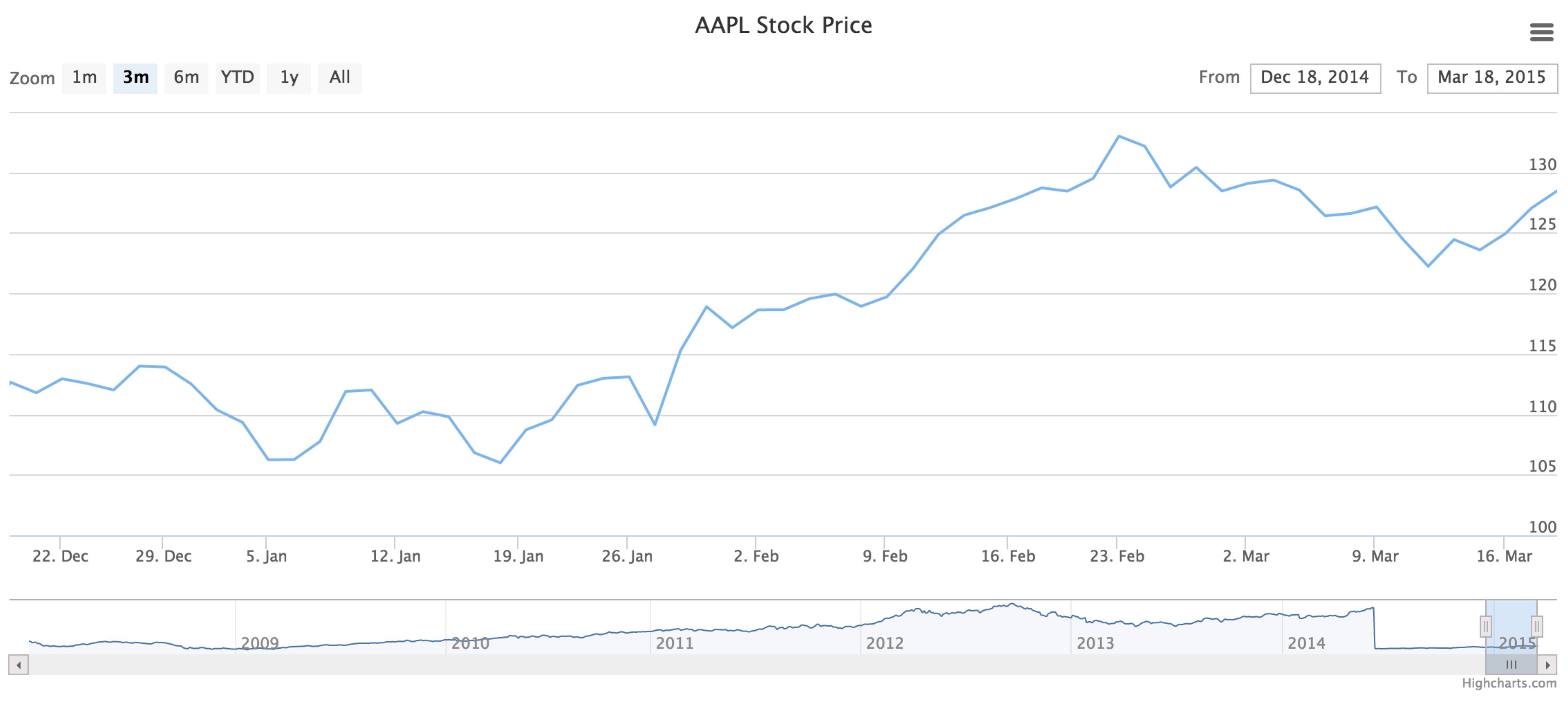
Now that we’re warmed up, let's try a more interesting example. Here the browser will ask the q server to call out to the Yahoo Finance site and retrieve historical stock price and volume data for Apple. The browser will then use the publicly available High Charts package to display a spiffy stock history graph. In this example there will be a bit more JavaScript and q, but it's tolerable. And again, no web server other than q.
First let's tackle the browser side. Save the following text file as ws101.html.
<!DOCTYPE HTML>
<html>
<head>
  <script src=
    "http://ajax.googleapis.com/ajax/libs/jquery/1.8.2/jquery.min.js">
  </script>
  <script src="http://code.highcharts.com/stock/highstock.js"></script>
  <script src=
    "http://code.highcharts.com/stock/modules/exporting.js"></script>
</head>
<body>
  <div id="container" style="height: 500px; min-width: 500px"></div>
</body>
<script src="c.js"></script>
<script>
  var serverurl = "//localhost:5042/",
    ws,
    c = connect(),
    ticker = "AAPL",
    startdt = "2008-01-01";

  function connect() {
    if ("WebSocket" in window) {
      ws=new WebSocket("ws:" + serverurl);
      ws.binaryType="arraybuffer";
      ws.onopen=function(e){
        toQ([ticker, startdt]);
      };
      ws.onclose=function(e){
      };
      ws.onmessage=function(e){
        return fromQ(e.data);
      };
      ws.onerror=function(e) {window.alert("WS Error") };
    } else alert("WebSockets not supported on your browser.");
  }

  function toQ(pl) {
    ws.send(serialize({ payload: pl }));
  }

  function fromQ(raw) {
    var data = deserialize(raw);
    return createChart(data);
  }

  function toUTC(x) {
    var y = new Date(x);
    y.setMinutes(y.getMinutes() + y.getTimezoneOffset());
    return y.getTime();
  }

  function createChart(data) {
    $('#container').highcharts('StockChart', {
      rangeSelector : {
        selected : 1
      },
      title : {
        text : ticker + ' Stock Price'
      },
      series : [{
        name : ticker,
        data : data.hist.map(function(x){return [toUTC(x.Date), x.Close]}),
        tooltip: {
          valueDecimals: 2
        }
      }]
    });
  }
</script>
</html>
We provide a concise description of the highlights, assuming familiarity with basic HTML5 and JavaScript.
- Load external scripts from Google (for JQuery) and High Charts (for the actual graphical display).
- Specify a simple HTML element to contain the actual graph.
- Load the local KX file
c.jsfor q serialization/deserialization. - Create the connection by calling
connect(), which assigns a handler foronopenthat callstoQwith the data variables. - Assign a handler to
onmessagethat passes the message tofromQ. - Initialize the variables that specify the historical data we will request from Yahoo Finance.
- The
toQfunction wraps its parameter in a JavaScript object, serializes it and (asynchronously) sends it to the q process where it will manifest as a serialized dictionary. - The
fromQfunction deserializes a received q dictionary, which magically becomes a JavaScript object, and passes it to thecreateChartfunction. - The auxiliary function
toUTCtransforms q dates to a form suitable for High Stocks. - The
createChartfunction instantiates a High Stocks stock price graph and populates the appropriate properties. Note the use ofmapto iterate over the individual time-series points; it is the functional programming equivalent ofeachin q. Also observe that we use the closing prices for the plot, as is customary.
The alignment between JavaScript objects and q dictionaries, along with built-in serialization/deserialization, makes data transfer between the browser and q effortless.
Now to the q server side, which has fewer lines of code that do much work. Save the following text file as ws101.q.
\p 5042

unixDate:{[dts] (prd 60 60 24)*dts-1970.01.01};

getHist:{[ticker; sdt; edt]
  tmpl:"https://query1.finance.yahoo.com/v7/finance/download/",
    "%tick?period1=%sdt&period2=%edt&interval=1d&events=history";
  args:enlist[ticker],string unixDate sdt,edt;
  url:ssr/[tmpl; ("%tick";"%sdt";"%edt"); args];
  / raw:system "wget -q -O - ",url;
  raw:system "curl -s '",url,"'";
  t:("DFFFFJF"; enlist ",") 0: raw;
  `Date xasc `Date`Open`High`Low`Close`Volume`AdjClose xcol t}

getData:{[ticker; sdt] select Date,Close from getHist[ticker;"D"$sdt;.z.D]}

.z.ws:{
  args:(-9!x) `payload;
  neg[.z.w] -8!(enlist `hist)!enlist .[getData; args; `err]}
Following is a description of the q code.
- Open port 5042
- Define the
unixDatefunction that converts dates to Unix timestamps. - Define the function
getHistthat does the real work. - Create a string template for the URL in which placeholders of the form
%argwill be replaced with specific values. - Run the start-date and end-date parameters through the date adjustment, stringify the results and concatenate onto the ticker string to form a list of actual argument strings for the URL.
- Use the Over operator
/withssr(string search and replace) and recursively replace each placeholder in the template with the corresponding stringified argument. - Instruct the OS to make a
curlweb call to the fully-specified Yahoo Finance URL. This returns raw time-series data as comma-separated string records with column headers in the first row. - Parse the text data into a table with the appropriate data types.
- Rename the columns suitably for user display, sort by date (just in case) and return the result.
The final entry in the q script sets the WebSockets handler. Here is its behavior.
- Deserialize the passed JavaScript object into a q dictionary and extract the payload field.
- Perform protected evaluation of the multi-variate
getHistfunction on the passed arguments. - Serialize the resulting timeseries table and asynchronously send it to the browser, where it appears as a serialized list of JavaScript objects, one for each day.
The Yahoo API changed in 2017. The code above has been revised and works as of 2020.06.28. [Ed.]
To run this example, start a fresh q process and load the ws101.q script.
q) \l /pages/ws101.qNow point your browser at
file:///pages/ws101.html
Wait a few seconds (depending on the speed of your internet connection) and – voilà! – you have a nifty graph of AAPL stock price.