White paper

Machine learning:
Using embedPy to apply LASSO regression

by Samantha Gallagher

From its deep roots in financial technology KX is expanding into new fields. It is important for q to communicate seamlessly with other technologies. The embedPy interface allows this to be done with Python.

The interface allows the kdb+ interpreter to manipulate Python objects, call Python functions, and load Python libraries. Developers can fuse the technologies, allowing seamless application of q’s high-speed analytics and Python’s extensive libraries.

This white paper introduces embedPy, covering both a range of basic tutorials as well as a comprehensive solution to a machine-learning project.

EmbedPy is available on GitHub for use with kdb+ V3.5+ and

• Python 3.5+ on macOS or Linux
• Python 3.6+ on Windows

The installation directory also contains a README.txt about embedPy, and a directory of detailed examples.

EmbedPy basics

In this section, we introduce some core elements of embedPy that will be used in the LASSO regression problem that follows.

Installing embedPy in kdb+

Download the embedPy package from GitHub: KxSystems/embedPy

Follow the instructions in README.md for installing the interface. Load p.q into kdb+ through either:

• the command line: $ q p.q
• the q session: q)\l p.q

Executing Python code from a q session

Python code can be executed in a q session by either using the p) prompt, or the .p namespace:

q)p)def add1(arg1): return arg1+1
q)p)print(add1(10))
11
q).p.e"print(add1(5))"
6
q).p.qeval"add1(7)"                       / print Python result
8

Interchanging variables

Python objects live in the embedded Python memory space. In q, these are foreign objects that contain pointers to the Python objects. They can be stored in q as variables, or as parts of lists, tables, and dictionaries, and will display foreign when inspected in the q console. Foreign objects cannot be serialized by kdb+ or passed over IPC; they must first be converted to q.

This example shows how to convert a Python variable into a foreign object using .p.pyget. A foreign object can be converted into q by using .p.py2q:

q)p)var1=2
q).p.pyget`var1
foreign
q).p.py2q .p.pyget`var1
2

Foreign objects

Whilst foreign objects can be passed back and forth between q and Python and operated on by Python, they cannot be operated on by q directly. Instead, they must be converted to q data. To make it easy to convert back and forth between q and Python representations a foreign object can be wrapped as an embedPy object using .p.wrap

q)p:.p.wrap .p.pyget`var1
q)p
{[f;x]embedPy[f;x]}[foreign]enlist

Given an embedPy object representing Python data, the underlying data can be returned as a foreign object or q item:

q)x:.p.eval"(1,2,3)"                / Define Python object
q)x
{[f;x]embedPy[f;x]}[foreign]enlist
q)x`.                               / Return the data as a foreign object
foreign
q)x`                                / Return the data as q
1 2 3

Edit Python objects from q

Python objects are retrieved and executed using .p.get. This will return either a q item or foreign object. There is no need to keep a copy of a Python object in the q memory space; it can be edited directly.

The first parameter of .p.get is the Python object name, and the second parameter is either < or >, which will return q or foreign objects respectively. The following parameters will be the input parameters to execute the Python function.

This example shows how to call a Python function with one input parameter, returning q:

q)p)def add2(x): res = x+2; return(res);
q).p.get[`add2;<]                    / < returns q
k){$[isp x;conv type[x]0;]x}.[code[code;]enlist[;;][foreign]]`.p.q2pargsenlist
q).p.get[`add2;<;5]                  / get and execute func, return q
7
q).p.get[`add2;>;5]                  / get execute func, return foreign object
foreign
q)add2q:.p.get`add2                  / define as q function, return an embedPy object
q)add2q[3]`                          / call function, and convert result to q
5

Python keywords

EmbedPy allows keyword arguments to be specified, in any order, using pykw:

q)p)def times_args(arg1, arg2): res = arg1 * arg2; return(res)
q).p.get[`times_args;<;`arg2 pykw 10; `arg1 pykw 3]
30

Importing Python libraries

To import an entire Python library, use .p.import and call individual functions:

q)np:.p.import`numpy
q)v:np[`:arange;12]
q)v`
0 1 2 3 4 5 6 7 8 9 10 11

Individual packages or functions are imported from a Python library by specifying them during the import command.

q)arange:.p.import[`numpy]`:arange    / Import function
q)arange 12
{[f;x]embedPy[f;x]}[foreign]enlist
q)arange[12]`
0 1 2 3 4 5 6 7 8 9 10 11
q)p)import numpy as np                # Import package using Python syntax
q)p)v=np.arange(12)
q)p)print(v)
[ 0 1 2 3 4 5 6 7 8 9 10 11]
q)stats:.p.import[`scipy.stats]       / Import package using embedPy syntax
q)stats[`:skew]
{[f;x]embedPy[f;x]}[foreign]enlist

Applying LASSO regression for analyzing housing prices

This analysis uses LASSO regression to determine the prices of homes in Ames, Iowa. The dataset used in this demonstration is the Ames Housing Dataset, compiled by Dean De Cock for use in data-science education. It contains 79 explanatory variables describing various aspects of residential homes which influence their sale prices.

kaggle.com

The Least Absolute Shrinkage and Selection Operator (LASSO) method was used for the data analysis. LASSO is a method that improves the accuracy and interpret-ability of multiple linear regression models by adapting the model fitting process to use only a subset of relevant features.

It performs L1 regularization, adding a penalty equal to the absolute value of the magnitude of coefficients, which reduces the less-important features’ coefficients to zero. This leaves only the most relevant feature vectors to contribute to the target (sale price), which is useful given the high dimensionality of this dataset.

A kdb+ Jupyter notebook on GitHub accompanies this paper.

kxcontrib/embedpy-lasso

Cleaning and pre-processing data in kdb+

Load data

As the data are stored in CSVs, the standard kdb+ method of loading a CSV is used. The raw dataset has column names beginning with numbers, which kdb+ will not allow in queries, so the columns are renamed on loading.

ct:"IISIISSSSSSSSSSSSIIIISSSSSISSSSSSSISIII"      / column types
ct,:"SSSSIIIIIIIIIISISISSISIISSSIIIIIISSSIIISSF"
train:(ct;enlist csv) 0:`: train.csv
old:`1stFlrSF`2ndFlrSF`3SsnPorch                  / old column names
new:`firFlrSF`secFlrSF`threeSsnPorch              / new column names
train:@[cols train; where cols[train] in old; :; new] xcol train

Log-transform the sale price

The sale price is log-transformed to obtain a simpler relationship of data to the sale price.

update SalePrice:log SalePrice from `train
y:train.SalePrice

Clean data

Cleaning the data involves several steps. First, ensure that there are no duplicated data, and then remove outliers as suggested by the dataset’s author.

q)count[train]~count exec distinct Id from train
1b
q)delete Id from `train
q)delete from `train where GrLivArea > 4000

Nxext, null data points within the features are assumed to mean that it does not have that feature. Any `NA values are filled with `No or `None, depending on category.

updateNulls:{[t]
  noneC:`Alley`MasVnrType;
  noC:`BsmtQual`BsmtCond`BsmtExposure`BsmtFinType1`BsmtFinType2`Fence`FireplaceQu;
  noC,:`GarageType`GarageFinish`GarageQual`GarageCond`MiscFeature`PoolQC;
  a:raze{y!{(?;(=;enlist`NA;y);enlist x;y)}[x;]each y}'[`None`No;(noneC;noC)];
  ![t;();0b;a]}

train:updateNulls train

Convert some numerical features into categorical features, such as mapping months and sub-classes. This is done for one-hot encoding later.

monthDict:(1+til 12)!`Jan`Feb`Mar`Apr`May`Jun`Jul`Aug`Sep`Oct`Nov`Dec
@[`train;`MoSold;monthDict]
subclDict:raze {enlist[x]!enlist[`$"SC",string[x]]}
  each 20 30 40 45 50 60 70 75 80 85 90 120 160 180 190
@[`train;`MSSubClass;subclDict]

Convert some categorical features into numerical features, such as assigning grading to each house quality, encoding as ordered numbers. These fields were selected for numerical conversion as their categorical values are easily mapped intuitively, while other fields are less so.

@[`train;;`None`Grvl`Pave!til 3] each `Alley`Street
quals: `BsmtCond`BsmtQual`ExterCond`ExterQual`FireplaceQu
quals,:`GarageCond`GarageQual`HeatingQC`KitchenQual
@[`train;;`No`Po`Fa`TA`Gd`Ex!til 6] each quals
@[`train;`BsmtExposure;`No`Mn`Av`Gd!til 4]
@[`train;;`No`Unf`LwQ`Rec`BLQ`ALQ`GLQ!til 7] each `BsmtFinType1`BsmtFinType2
@[`train;`Functional;`Sal`Sev`Maj2`Maj1`Mod`Min2`Min1`Typ!1+til 8]
@[`train;`LandSlope;`Sev`Mod`Gtl!1+til 3]
@[`train;`LotShape;`IR3`IR2`IR1`Reg!1+til 4]
@[`train;`PavedDrive;`N`P`Y!til 3]
@[`train;`PoolQC;`No`Fa`TA`Gd`Ex!til 5]
@[`train;`Utilities;`ELO`NoSeWa`NoSewr`AllPub!1+til 4]

Feature engineering

To increase the model’s accuracy, some features are simplified and combined based on similarities. This is done in three steps demonstrated below.

Simplification of existing features

Some numerical features’ scopes are reduced, and several categorical features are mapped to become simple numerical features.

ftrs:`OverallQual`OverallCond`GarageCond`GarageQual`FireplaceQu`KitchenQual
ftrs,:`HeatingQC`BsmtFinType1`BsmtFinType2`BsmtCond`BsmtQual`ExterCond`ExterQual
rng:(1+til 10)!1 1 1 2 2 2 3 3 3 3
{![`train;();0b;enlist[`$"Simpl",string[x]]!enlist (rng;x)]} each ftrs
rng:(1+til 8)!1 1 2 2 3 3 3 4
{![`train;();0b;enlist[`$"Simpl",string[x]]!enlist (rng;x)]} each `PoolQC`Functional

Combination of existing features

Some of the features are very similar and can be combined into one. For example, Fireplaces and FireplaceQual can become one overall feature of FireplaceScore.

gradeFuncPrd:{[t;c1;c2;cNew]![t;();0b;enlist[`$string[cNew]]!enlist (*;c1;c2)]}

combineFeat1:`OverallQual`GarageQual`ExterQual`KitchenAbvGr,
  `Fireplaces`GarageArea`PoolArea`SimplOverallQual`SimplExterQual,
  `PoolArea`GarageArea`Fireplaces`KitchenAbvGr

combineFeat2:`OverallCond`GarageCond`ExterCond`KitchenQual,
  `FireplaceQu`GarageQual`PoolQC`SimplOverallCond`SimplExterCond,
  `SimplPoolQC`SimplGarageQual`SimplFireplaceQu`SimplKitchenQual

combineFeat3:`OverallGrade`GarageGrade`ExterGrade`KitchenScore,
  `FireplaceScore`GarageScore`PoolScore`SimplOverallGrade`SimplExterGrade,
  `SimplPoolScore`SimplGarageScore`SimplFireplaceScore`SimplKitchenScore;

train:train{gradeFuncPrd[x;]. y}/flip(combineFeat1; combineFeat2; combineFeat3)

update TotalBath:BsmtFullBath+FullBath+0.5*BsmtHalfBath+HalfBath,
  AllSF:GrLivArea+TotalBsmtSF,
  AllFlrsSF:firFlrSF+secFlrSF,
  AllPorchSF:OpenPorchSF+EnclosedPorch+threeSsnPorch+ScreenPorch,
  HasMasVnr:((`BrkCmn`BrkFace`CBlock`Stone`None)!((4#1),0))[MasVnrType],
  BoughtOffPlan:((`Abnorml`Alloca`AdjLand`Family`Normal`Partial)!((5#0),1))[SaleCondition]
  from `train

Use correlation (cor) to find the features that have a positive relationship with the sale price. These will be the most important features relative to the sale price, as they become more prominent with an increasing sale price.

q)corr:desc raze {enlist[x]!enlist train.SalePrice cor ?[train;();();x]} 
  each exec c from meta[train] where not t="s"

q)10#`SalePrice _ corr  / Top 10 most relevant features
OverallQual     | 0.8192401
AllSF           | 0.8172716
AllFlrsSF       | 0.729421
GrLivArea       | 0.7188441
SimplOverallQual| 0.7079335
ExterQual       | 0.6809463
GarageCars      | 0.6804076
TotalBath       | 0.6729288
KitchenQual     | 0.6671735
GarageScore     | 0.6568215

Polynomials on the top ten existing features

Create new polynomial features from the top ten most relevant features. These mathematically derived features will improve the model by increasing flexibility. Polynomial regression is used as it describes the relationship between the data and sale price most accurately.

polynom:{[t;c]
  a:raze(!).'(
    {`$string[x] ,/:("_2";"_3";"_sq")}; 
    {((xexp;x;2);(xexp;x;3);(sqrt;x))}
  )@\:/:c;
  ![t;();0b;a]}

train:polynom[train;key 10#`SalePrice _ corr]

Handling categorical and numerical features separately

Split the dataset into numerical features (minus the sale price) and categorical features.

.feat.categorical:?[train;();0b;]{x!x} 
  exec c from meta[train] where t="s"

.feat.numerical:?[train;();0b;]{x!x} 
  (exec c from meta[train] where not t="s") except `SalePrice

Numerical features

Fill nulls with the median value of the column:

![`.feat.numerical;();0b;{x!{(^;(med;x);x)}each x}cols .feat.numerical]

Outliers in the numerical features are assumed to have a skewness of >0.5. These are log-transformed to reduce their impact:

skew:.p.import[`scipy.stats;`:skew] / import Python skew function
skewness:{skew[x]`}each flip .feat.numerical
@[`.feat.numerical;where abs[skewness]>0.5;{log[1+x]}]

Categorical features

Create dummy features via one-hot encoding, then join with numerical results for complete dataset.

oneHot:{[pvt;t;clm]
  t:?[t;();0b;{x!x}enlist[clm]];
  prePvt:![t;();0b;`name`true!(($;enlist`;((/:;,);string[clm],"_";($:;clm)));1)];
  pvtCol:asc exec distinct name from prePvt;
  pvtTab:0^?[prePvt;();{x!x}enlist[clm];(#;`pvtCol;(!;`name;`true))];
  pvtRes:![t lj pvtTab;();0b;enlist clm];$[()~pvt;pvtRes;pvt,'pvtRes]}

train:.feat.numerical,'()oneHot[;.feat.categorical;]/cols .feat.categorical

Modeling

Splitting data

Partition the dataset into training sets and test sets by extracting random rows. The training set will be used to fit the model, and the test set will be used to provide an unbiased evaluation of the final model.

trainIdx:-1019?exec i from train // training indices
X_train:train[trainIdx]
yTrain:y[trainIdx]
X_test:train[(exec i from train) except trainIdx]
yTest:y[(exec i from train) except trainIdx]

Standardize numerical features

Standardization is done after the partitioning of training and test sets to apply the standard scalar independently across both. This is done to produce more standardized coefficients from the numerical features.

stdSc:{(x-avg x) % dev x}
@[`X_train;;stdSc] each cols .feat.numerical
@[`X_test;;stdSc] each cols .feat.numerical

Transform kdb+ tables into Python-readable matrices

xTrain:flip value flip X_train
xTest:flip value flip X_test

Analysis using embedPy

This section analyses the data using several Python libraries from inside the q process: pandas, NumPy, sklearn and Matplotlib.

Import Python libraries

pd:.p.import`pandas
np:.p.import`numpy
cross_val_score:.p.import[`sklearn.model_selection;`:cross_val_score]
qLassoCV:.p.import[`sklearn.linear_model;`:LassoCV]

Train the LASSO model

Create NumPy arrays of kdb+ data:

arrayTrainX:np[`:array][0^xTrain] 
arrayTrainY:np[`:array][yTrain]
arrayTestX: np[`:array][0^xTest]
arrayTestY: np[`:array][yTest]

Use pykw to set alphas, maximum iterations, and cross-validation generator.

qLassoCV:qLassoCV[
  `alphas pykw (.0001 .0003 .0006 .001 .003 .006 .01 .03 .06 .1 .3 .6 1); 
  `max_iter pykw 50000; 
  `cv pykw 10; 
  `tol pykw 0.1]

Fit linear model using training data, and determine the amount of penalization chosen by cross-validation (sum of absolute values of coefficients). This is defined as alpha, and is expected to be close to zero given LASSO’s shrinkage method:

q)qLassoCV[`:fit][arrayTrainX;arrayTrainY]
q)alpha:qLassoCV[`:alpha_]`
q)alpha
0.01

Define the error measure for official scoring: Mean squared error (MSE)

The MSE is commonly used to analyze the performance of statistical models utilizing linear regression. It measures the accuracy of the model and is capable of indicating whether removing some explanatory variables is possible without impairing the model’s predictions. A value of zero measures perfect accuracy from a model. The MSE will measure the difference between the values predicted by the model and the values actually observed. MSE scoring is set in the qLassoCV function using pykw, which allows individual keywords to be specified.

crossValScore:.p.import[`sklearn;`:model_selection;`:cross_val_score]
mseCV:{crossValScore[qLassoCV;x;y;`scoring pykw `neg_mean_squared_error]`}

The average of the MSE results shows that there are relatively small error measurements from this model.

q)avg mseCV[np[`:array][0^xTrain];np[`:array][yTrain]]
-0.1498252

Find the most important coefficients

q)impCoef:desc cols[train]!qLassoCV[`:coef_]`
q)count where value[impCoef]=0
284
q)(5#impCoef),-5#impCoef
TotalBsmtSF | 0.05086288
GrLivArea   | 0.02549123
OverallCond | 0.02080637
TotalBath_sq| 0.01637903
PavedDrive  | 0.01415822
LandSlope   | -0.009958406
BsmtFinType2| -0.01045939
KitchenAbvGr| -0.01527232
Street      | -0.01618361
LotShape    | -0.02050625

As seen above, LASSO eliminated 284 features, and therefore only used one-tenth of the features. The most influential coefficients show that LASSO gives higher weight to the overall size and condition of the house, as well as some land and street characteristics, which intuitively makes sense. The total square foot of the basement area (TotalBsmtSF) has a large positive impact on the sale price, which seems unintuitive, but could be correlated to the overall size of the house.

Prediction results

lassoTest:qLassoCV[`:predict][arrayTestX]

The image lassopred.png illustrates the predicted results, plotted on a scatter graph using Matplotlib:

qplt:.p.import[`matplotlib.pyplot];

ptrain:qLassoCV[`:predict][arrayTrainX];
ptest: qLassoCV[`:predict][arrayTestX];

qplt[`:scatter]
  [ptrain`;
   yTrain;
   `c      pykw "blue";
   `marker pykw "s";
   `label  pykw "Training Data"];
qplt[`:scatter];
  [ptest`;
   yTest;
   `c      pykw "lightgreen";
   `marker pykw "s";
   `label  pykw "Validation Testing Data"];

qplt[`:title]"Linear regression with Lasso regularization";
qplt[`:xlabel]"Predicted values";
qplt[`:ylabel]"Real values";
qplt[`:legend]`loc pykw "upper left";

bounds:({floor min x};{ceiling max x})@\:/:raze 
  each((ptrain`;ptest`);(yTrain;yTest));
bounds:4#bounds first idesc{abs x-y}./:bounds;
qplt[`:axis]bounds;

qplt[`:savefig]"lassopred.png";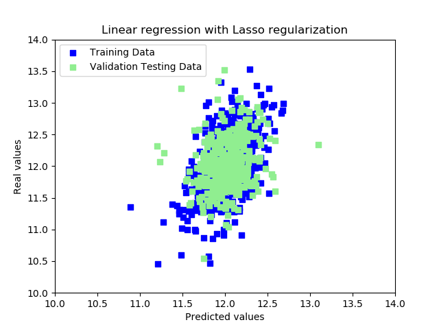

Conclusion

In this white paper, we have shown how easily embedPy allows q to communicate with Python and its vast range of libraries and packages. We saw how machine-learning libraries can be coupled with q’s high-speed analytics to significantly enhance the application of solutions across big data stored in kdb+. Python’s keywords can be easily communicated across functions using the powerful pykw, and visualization tools such as Matplotlib can create useful graphics of kdb+ datasets and analytics results. Also demonstrated was how q’s vector-oriented nature is optimal for cleaning and pre-processing big datasets.

This interface is useful across many institutions that are developing in both languages, allowing for the best features of both technologies to fuse into a powerful tool. Further machine-learning techniques powered by kdb+ can be found under Featured Resources at kx.com/machine-learning.

PDF

Author

Samantha (Gallagher) Devlin has worked on implementing kdb+ solutions for financial institutions globally.    

Other papers by Samantha Gallagher

• kdb+ and Microsoft Azure
• Free byte-sized kdb+ training
• We DARE you to learn about kdb+ encryption