Data sources#
A data source is used to retrieve data, from connected databases, for use by dashboard components. This page describes the following.
- Creating data sources
- Creating data source queries, using kdb+/q, SQL, python and more
- Configuring data source connections
- Setting data source subscription types
- Additional data source configuration including, auto-execute and max rows
- Configuring pivot queries for pivot grid components
- Configuring update queries to make permanent changes to source data from the data grid component
- Viewing results, and mapping results from a data source to view states
Configure a data source#
To configure a component's data source:
-
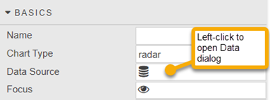
Open the Data dialog, as shown below, by either:
-
Clicking on the database icon
 at the top of the properties panel or
-
Clicking the component’s Data Source property. Note that this property can be in different property sections for different components. In this example it is in the Basics properties.
-
-
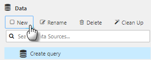
Click New to create a new data source and give it a name.
-
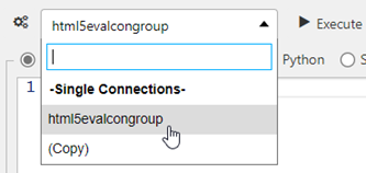
Select a connection or connection group, from the connection selector, as shown below.
-
Create a data source query, as described here.
-
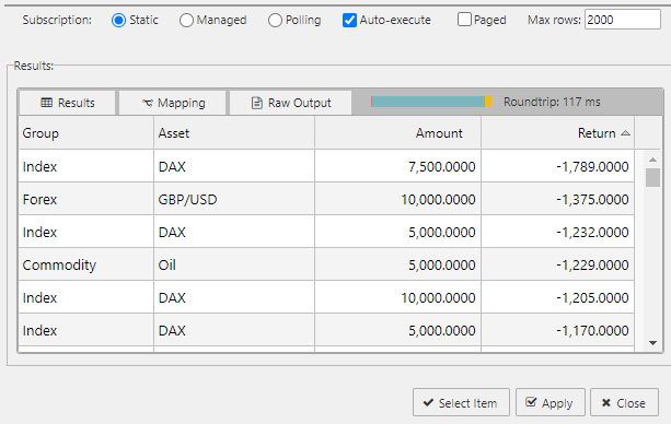
Click Execute to run the query. If the query is successful the Results table populates with the query results, as shown below. Otherwise an error is displayed. See here for more about results.
-
Click Apply to save the changes made to the data source and/or Select Item to choose the selected data source for the component property.
Create a data source query#
There are a variety of options for creating data source queries, as follows:
- SQL - to create a query using SQL query text. If this option is not available see here for how to get it.
- kdb+/q - to create a query using kdb+/q query text.
- Builder - to build a query using input nodes.
- Analytic - to pick from a pre-defined list of functions.
- Python - to build a python query. This option is greyed out if PyKX and dashboard specific PyKX dependencies are not installed.
- Streaming - to build a real-time streaming query.
- Virtual - to build a query using javascript.
SQL#
SQL Availability
Please note that the SQL query functionality is not available by default. To access this feature:
- Licensed users contact your account executive for more information.
- Free Trial users install either kdb Insights Personal Edition or kdb Insights Core
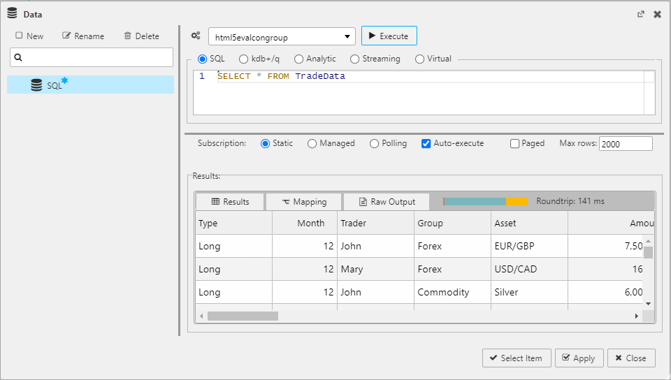
SQL queries use text-based SQL to query data from the database. Enter the following SQL query in the SQL tab of the Data dialog.
SELECT * FROM TradeData
The following screenshot displays this simple SQL query which returns all column data in the TradeData table from the html5evalcongroup connection.
kdb+/q#
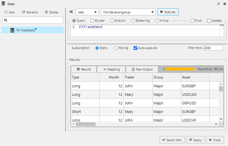
You can use text-based q to query data from the database. For example enter the following in the kdb+/q query screen:
FXTradeData
The following screenshot shows this simple q query which returns all column data in FXTradeData table from the html5evalcongroup connection.
Builder#
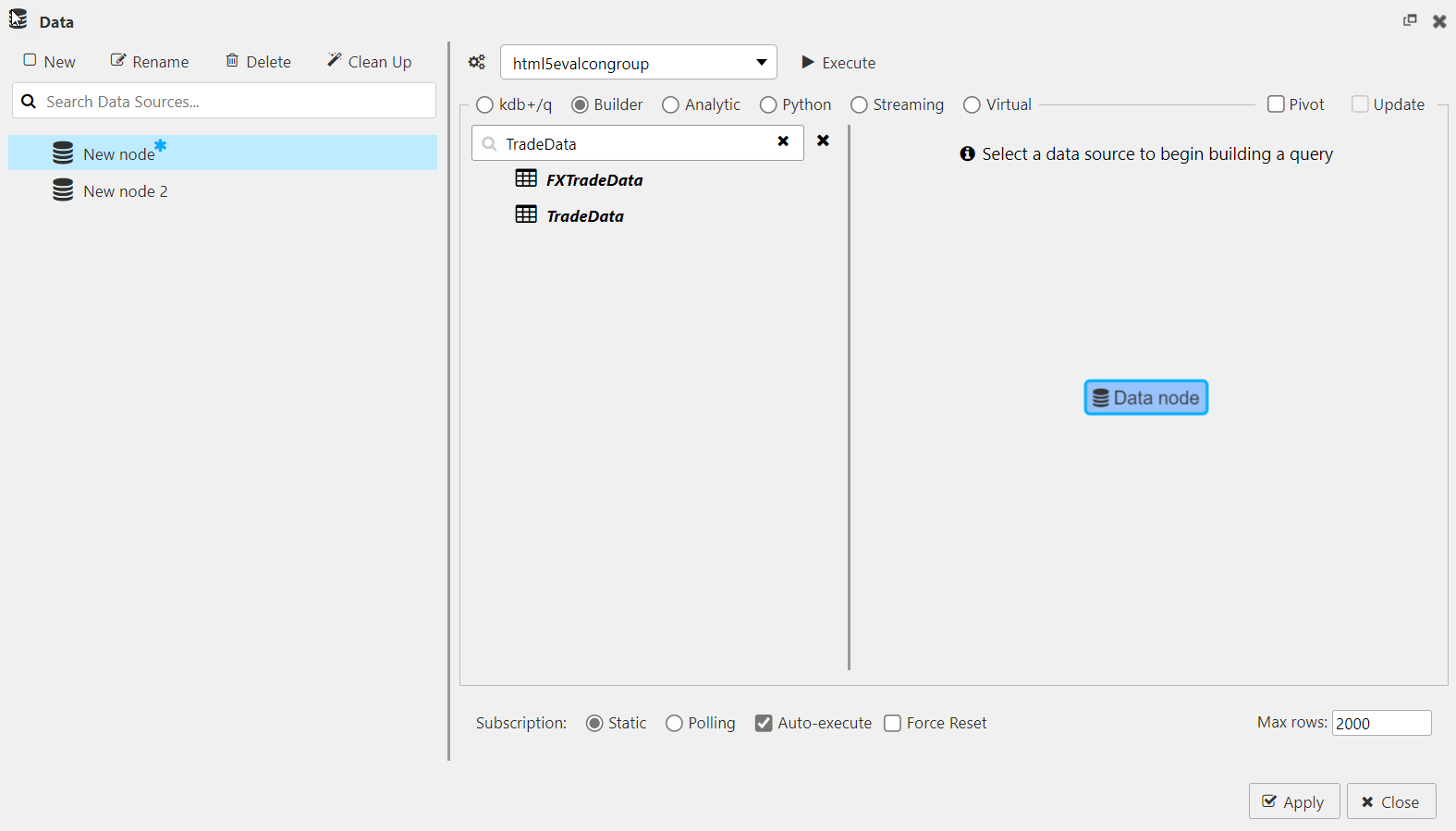
Visual queries allow dashboard users, with no programming experience, to build queries using a range of configurable dialogs.
-
Select Builder and expand the editor to full screen mode
 .
. -
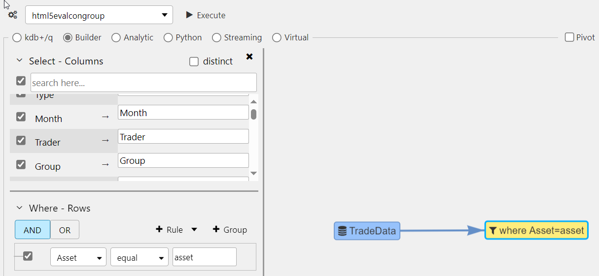
Select a data node in the menu of available data sources. You can type in the name of the node in the search box as in the following example, where the TradeData node is entered and selected.
-
Right-click on an existing node to add one of the following:
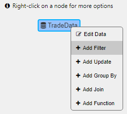
-
Each node-type displays its own unique dialog used to define the query, as illustrated below.
-
Queries can be linked to view state parameters. For example, the filter node below has a Where clause that filters for items equal to the View State parameter Asset.
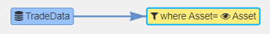
-
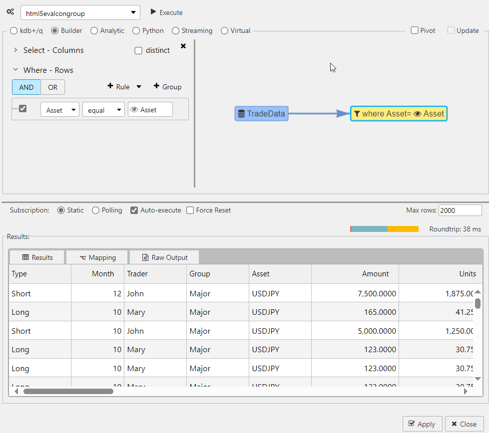
Click Execute to run the query. Then click Apply or Close.
Streaming query#
Static and real-time data can be combined where data shares the same node. The following example connects static fundamental data for equities to streaming equity prices, using the ticker symbol as a join between the data sets. This data is available when you install KX Dashboards.
-
In the Data dialog select Builder and search and select the streaming data source list. The parameter x can be left unassigned as this is handled by the join.
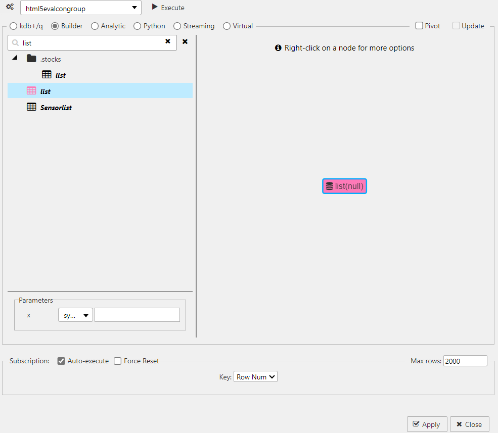
In the Data editor, streaming data sources have a colored icon and static data sources are black.
-
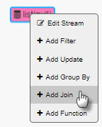
Right-click on list node and select Add Join, as shown below.
-
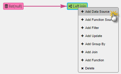
For the join node, right-click to Add Data Source, as shown below.
-
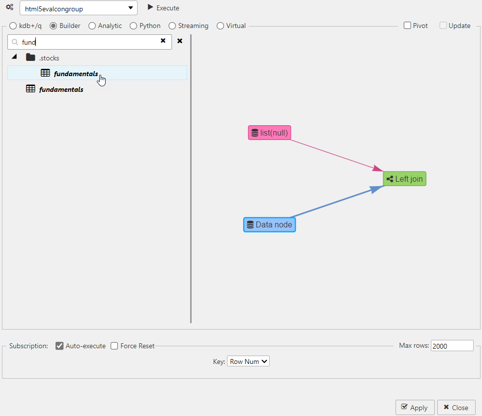
Select fundamentals from the Stocks folder, as shown below. This is a static data source of stock fundamentals.
-
Define how the data sources are connected. There has to be a common key between each data source to create the join, in this case, sym.
- Left click on the Left Join node and click Edit Join.
-
Check the key which connects the two data sources; only shared keys are selectable. A left join adds content matched by the key from the right table to the left table.
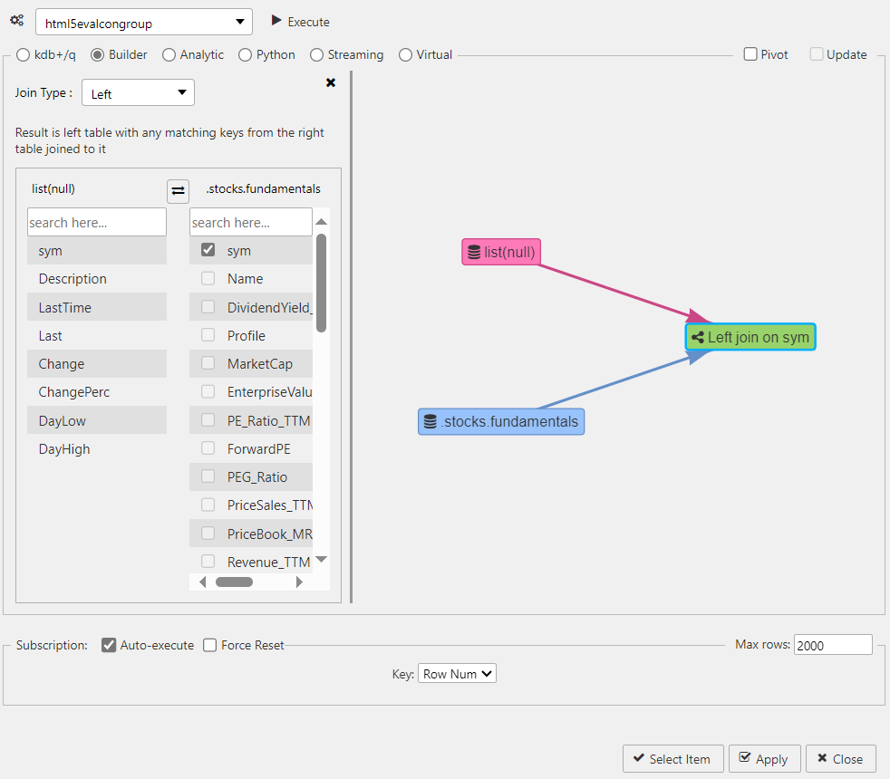
-
Click Execute to run the query.
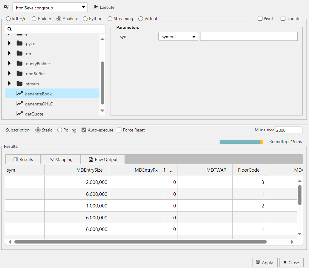
Analytic#
Analytics are pre-defined functions with required input parameters exposed in the dashboard. The following screenshot shows a sample analytic.
Analytics can be loaded directly into the q process There is sample analytics loaded as part of demo.q in the sample folder.
Python#
The option to write Python queries enhances KX Dashboards capabilities by leveraging the functionality of the PyKX library for interacting with kdb+/q databases.
Prerequisites
This functionality is supported for PyKX versions 2.3.1 or higher. To use python queries you must install PyKX and dashboard specific PyKX dependencies as follows:
To write Python queries:
-
Click the Python radio button in the Data dialog. If PyKX is not installed this option is greyed out.
-
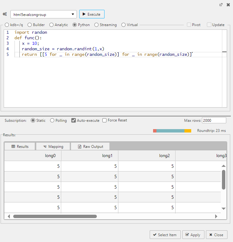
Enter the python query in the Python tab. For example enter the following query.
python
    import random
    def func():
        x = 10;
        random_size = random.randint(1,x)
        return [[5 for _ in range(random_size)] for _ in range(random_size)]
This simple Python function generates a random 2D list with dimensions NxN, where N is a random integer between 1 and 10 (inclusive). Each element in the list is set to the value 5.
Parsing logic
The parsing logic for the Python function string definition operates such that the first function that is defined within the code block is used as the callable function. Specifically this means that any import statements prior to the function definition are executed, usable and valid but any functions defined following the first function are ignored.
-
Click Execute and view the output in the Results panel, as shown below.
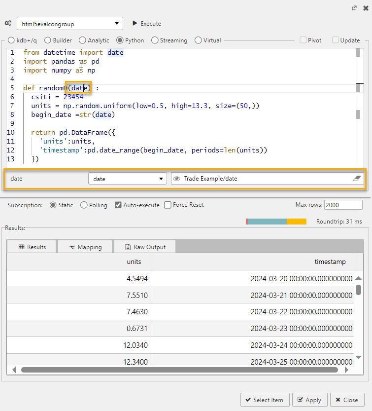
View States with python queries#
View states store values accessible to all components of the dashboard, click here to read more about view states.
You can use view states in Python queries. The following example shows the randomD function which generates a pandas DataFrame with random values and timestamps. The random values are uniformly distributed between 0.5 and 13.3, and the timestamps start from the given date, with the date being passed in as a view state.
You can use multiple view states by separating them with commas, as in (viewstate1, viewstate2, viewstate3). The following example shows 3 View States; sizeV, lowV, and highV.
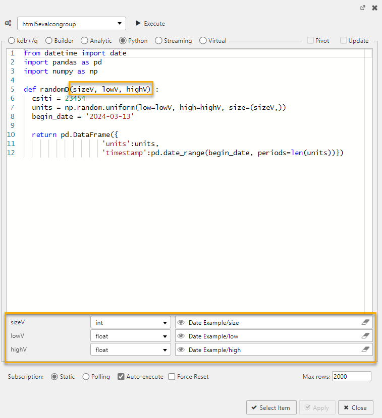
Note
The definition of Python functions and their use as view states presently only supports positional arguments as outlined above. Use of keyword arguments is not supported when defining Python functions.
Streaming#
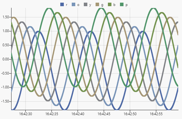
The following video describes the steps to create a kdb+ streaming process.
This section describes how to build a streaming, time series data set to display in a chart at 60 fps.
- Create a streaming q process on an assigned port; for example,
stream.qon port 6814:
`C:\User\Desktop\Direct\sample>q stream.q -p 6814`
stream.quses a sinewave to generate sample data over time:
/ define stream schema
waves:([]time:`timestamp$(); r:`float$(); o:`float$(); y:`float$(); g:`float$(); b:`float$(); p:`float$());

/ load and initialize kdb+tick
/ all tables in the top-level namespace (`.) become publish-able
\l tick/u.q
.u.init[];

/ sinwave
/ t, scalar t represents position along a single line
/ a, amplitude, the peak deviation of the function from zero
/ f, ordinary frequency, the number of oscillations (cycles) that occur each second of time
/ phase, specifies (in radians) where in its cycle the oscillation is at t = 0
.math.pi:acos -1;
.math.sineWave:{[t;a;f;phase] a * sin[phase+2*.math.pi*f*t] }

/ publish stream updates
.z.ts:{ .u.pub[`waves;enlist `time`r`o`y`g`b`p!(.z.p,{.math.sineWave[.z.p;1.4;1e-10f;x]-0.4+x%6} each til 6)] }
.u.snap:{waves} // reqd. by dashboards

\t 16

// ring buffer writes in a loop
.ringBuffer.read:{[t;i] $[i<=count t; i#t;i rotate t] }
.ringBuffer.write:{[t;r;i] @[t;(i mod count value t)+til 1;:;r];}

// cache updates for the snapshot
.stream.i:0-1;
.stream.waves:20000#waves;

// generate and save new record to buffer
.stream.wavesGen:{
    res: enlist `time`r`o`y`g`b`p!(.z.p,{(x%6)+.math.sineWave[.z.p;1.4;1e-10f;x] - 0.4} each til 6);
    .ringBuffer.write[`.stream.waves;res;.stream.i+:1];
    res
 }

/ generate & publish waves
.z.ts:{ .u.pub[`waves;.stream.wavesGen[]] }

// implement snapshot function
.u.snap:{[x] .ringBuffer.read[.stream.waves;.stream.i] }
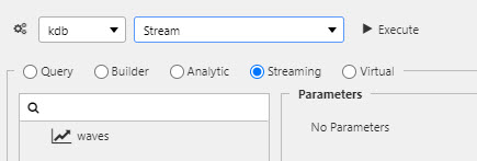
- Create a data connection in dashboards to the streaming process on the selected port.
- Select the data source, keyed by
time.
Virtual#
Virtual queries are built using Javascript and utilize data pre-loaded to the client. Assigned data sources in a virtual query do not re-query the database.
Virtual queries can meld data from more than one data source, view state parameter or text insert.
Virtual queries are not supported for the ChartGL component
Due to the processing optimizations inherent to ChartGL, the chartGL component does not currently support virtual queries
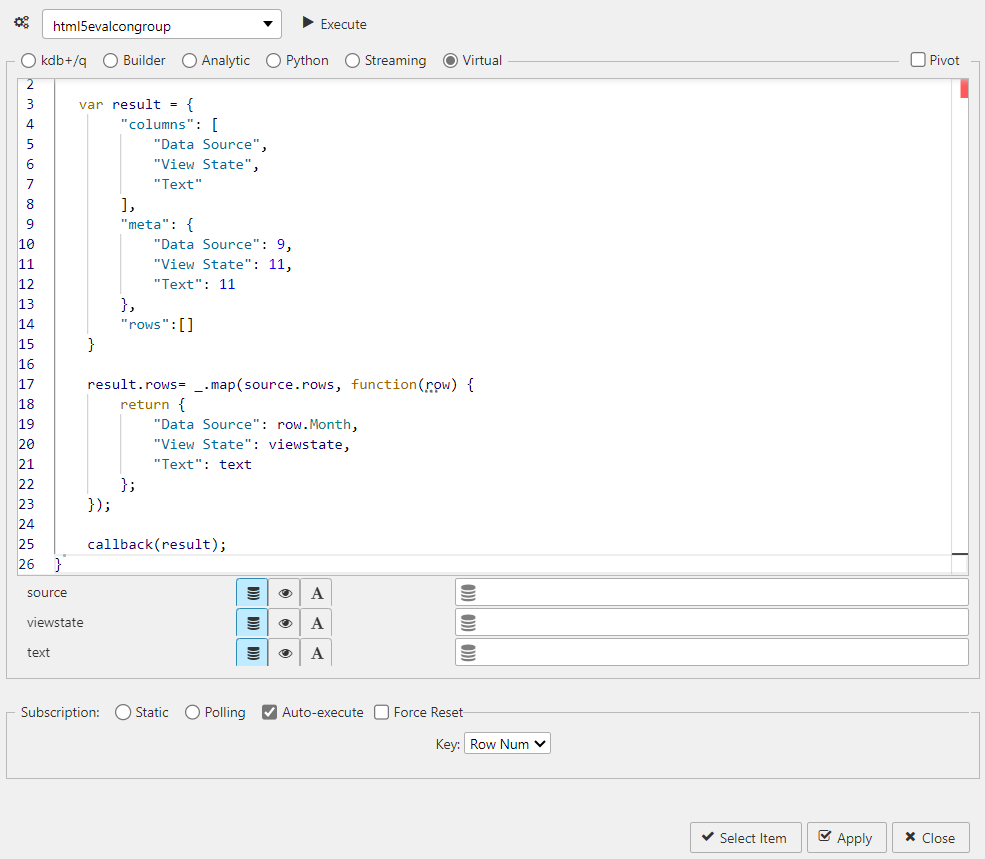
Select Virtual and enter the following Javascript.
function(source, viewstate, text, callback) {

   var result = {
        "columns": [
            "Data Source",
            "View State",
            "Text"
        ],
        "meta": {
            "Data Source": 9,
            "View State": 11,
            "Text": 11
        },
        "rows":[]
    }

    result.rows= _.map(source.rows, function(row) {
        return {
            "Data Source": row.Month,
            "View State": viewstate,
            "Text": text
        };
    });

    callback(result);
}
In this example, shown below, a result object is created with the following properties; columns (Data Source, View State and Text), meta and rows. Each row from the source.rows array is mapped to a new object with the specified properties:
- Data Source- Taken from the row.Month value.
- View State- Set to the view state provided.
- Text- Set to the text provided.
Meta definitions
The meta definitions are the kdb+ datatypes for each column where columns are the names of your table headers.
Rolling view states in data source queries#
For data sources with parameters, the parameter values that come from view states can instead come from their rolling syntax.
This feature is available with the following data source types: SQL, kdb+/q, Analytic, Python, Streaming and Virtual.
For example:
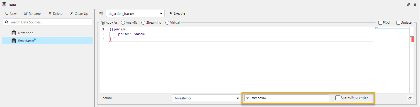
- Create a data source using a kdb+/q data query. Add a query that uses a parameter value and outputs the value of that parameter as shown below.
    {[param]
       param: param
    }

- Click on the eye icon to open the View State dialog.
-
Create a view state with rolling syntax as described here.
The following example shows a view state called tomorrow with rolling syntax of NOW+24:00.

-
Click Select Item to apply this to the data source.
-
The Data dialog is updated with the view state parameter and because this view state has rolling syntax a Use Rolling Syntax checkbox is now visible.
-
When you execute the query the value from the view state is used for the parameter input. The results shown vary, depending on whether Use Rolling Syntax is checked.
- Checked - The results show tomorrow's date (exactly 24 hours from now). If you Execute again the value updates to exactly 24 hours from the time you clicked Execute.
Additionally, when the rolling syntax is used for the parameter Value, the Value of the view state is also updated with the re-interpreted rolling syntax. - Unchecked - The results show the same date and time from the view state dialog. If you Execute again the value doesn't change.
- Checked - The results show tomorrow's date (exactly 24 hours from now). If you Execute again the value updates to exactly 24 hours from the time you clicked Execute.
-
Note that once you click Apply you cannot edit the Rolling Syntax status of the associated view state. If you attempt to edit the view state the Rolling Syntax checkbox is disabled because it is in use by a data source.
Subscriptions#
The following types of data source subscription are supported:
Static#
This is the default setting and involves a single request for data.
Polling#
Polling involves a client-side poll of the database. This is a direct client request to the database. Server paging can be enabled to limit the amount of data returned to the dashboard.
| Option | Effect |
|---|---|
| Interval | Time between client poll requests |
| Key | Select which data source column to define Subscription handling; e.g. to have continual or static update |
| Force Reset | By default, for updating data sources, KX Dashboards merges updates from the server with its existing dataset, unless a parameter is changed in which case the existing dataset is cleared. Enabling Force Reset clears the existing dataset each time it receives an update, regardless of whether a parameter has changed or not. |
Streaming#
Streaming subscriptions push data to the dashboard in place of a client or server-side poll.
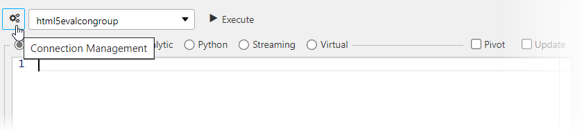
Connection Management#
Open the Connection Management screen by clicking on the Connection Management icon, shown below.
The *Connection Management screen has the following option:
- New - to create a new connection
- Duplicate - to create a copy of a selected connection
- Delete - to delete selected connection
- Save - to save details of connection
- Close - to close the window
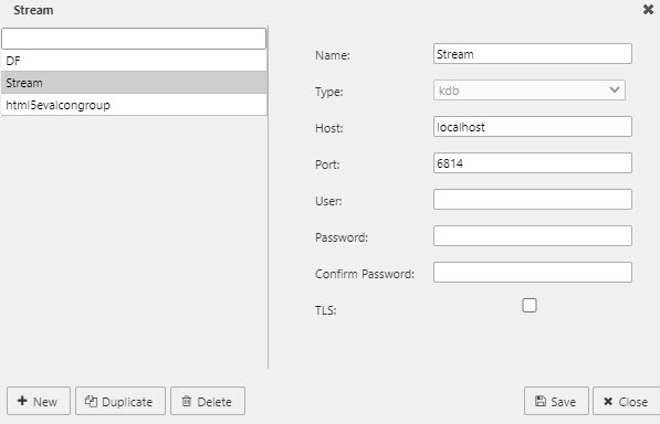
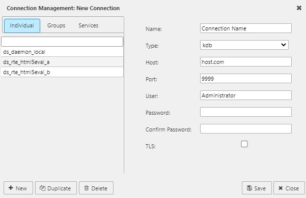
Create a connection#
To create a new connection, click New in the Connection Management screen. The connection properties, shown in the screenshot below, are as follows:
- Name - Enter a name for the connection.
- Type - The default and only option is kdb.
- Host/Port - Enter the server name or IP address of the connection host and the port to be used.
- User - The username is required when TLS is enabled.
- Password/Confirm Password - A password is required when TLS is enabled.
- TLS - Enabling Transport Layer Security (TLS) allows users to encrypt their kdb+ connection. kdb+ version 3.4 onwards supports TLS connections
Additional data source configuration#
Auto-execute#
This controls whether the data source automatically executes when an input parameter is changed or on load.

- Checked - The data source automatically executes whenever an input parameter is changed or on load if mapping is used. This is the default.
- Unchecked - Subsequent parameter changes do not execute the query. However, it still executes normally if associated with a component, e.g., a data grid on load, or as an action tied to a button.
Max Rows#
This specifies the max number of rows of data that can be returned for any subscription type. The default is 2,000 rows.
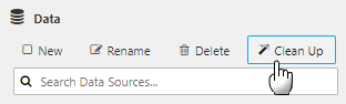
Clean Up#
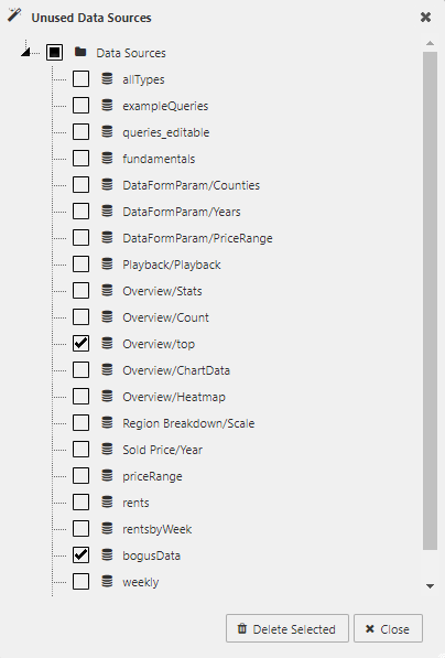
Click Clean Up to open the Unused Data Sources dialog, shown below.
This displays a list of data sources that are not being used by the dashboard. To remove one or more data source definitions:
- Tick the checkbox next to its name
- Click Delete Selected
- To select the entire list, check the topmost checkbox labeled Data Sources.
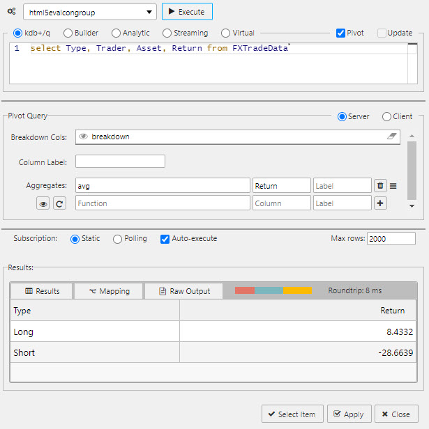
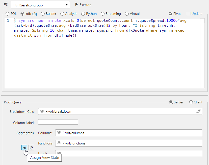
Pivot query#
Pivot queries are used by the Pivot Grid component.
Pivot data are split between independent variables (Breakdown Cols) and dependent variables (Aggregates). The following screenshot shows a pivot query.
Case-sensitive names
Names for Breakdown Cols and Aggregates are case-sensitive. If an error occurs, check that column-header names in the source database matches those used in the dashboard.
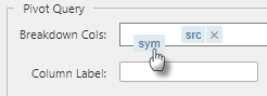
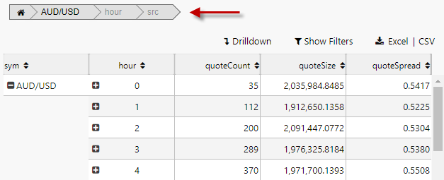
The order of the Breakdown Cols can be changed using drag-and-drop, as shown below.
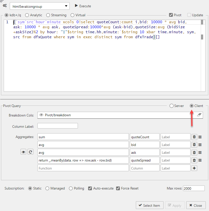
Client pivot#
In a server pivot the data request is processed server-side and only viewed data is returned to the dashboard. Each pivot interaction creates a fresh server-side request. A client pivot requests all data on dashboard load, and processes all pivot interactions on the client.
Use a server pivot for large data sets. For smaller data sets, a client pivot is faster. Click Client to create a client pivot as shown in the following screenshot.
Custom binary analytics and client pivots
As a client pivot is not making a server request for data, custom binary analytics aggregate functions using q do not operate. Use Javascript functions to build custom binary analytics aggregate functions for client pivots.
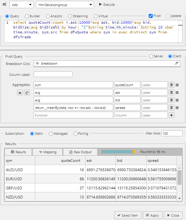
The following screenshot shows an example of a multi-column client pivot.
Pivot breakdown via breadcrumbs#
The order of the pivot breakdown can also be controlled by the dashboard end-user, with the Breadcrumbs component.
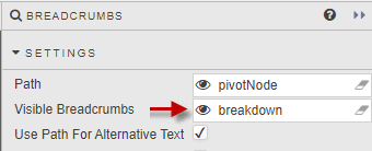
-
Create a View State Parameter (for example, breakdown) and associate it with the Visible Breadcrumbs property in the Breadcrumbs component’s Settings.
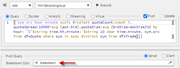
-
In the linked pivot query, set the Breakdown Cols to the breakdown view state parameter.
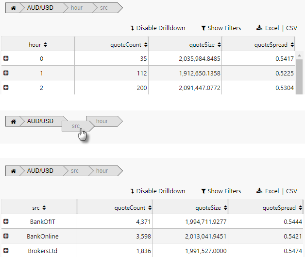
-
The resulting output shows the breakdown elements laid out in the Breadcrumb component. These can be dragged and repositioned to change the pivot order.
Column label#
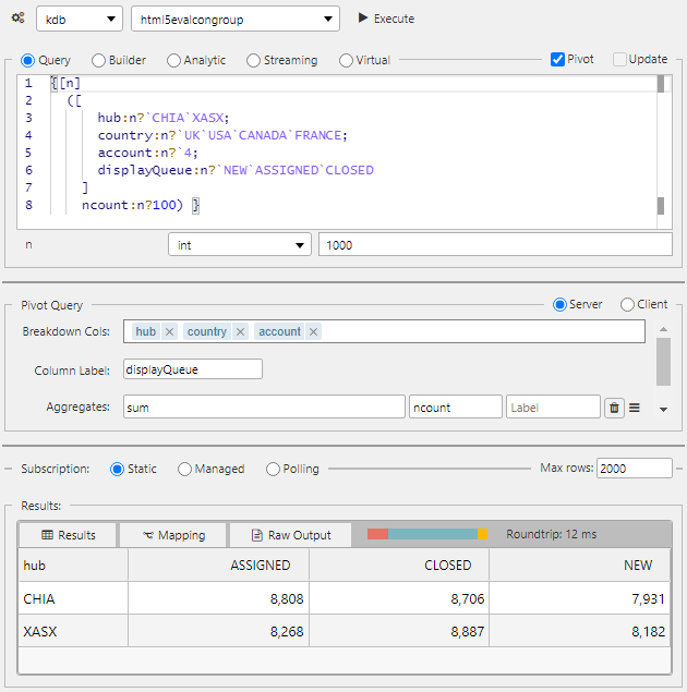
In the Pivot Query screen, Column Label can be used to support 2-dimensional pivots. For example enter the following two-dimensional pivot query in the Query tab.
{[n]
  ([
      hub:n?`CHIA`XASX;
      country:n?`UK`USA`CANADA`FRANCE;
      account:n?`4;
      displayQueue:n?`NEW`ASSIGNED`CLOSED
    ]
    ncount:n?100) }
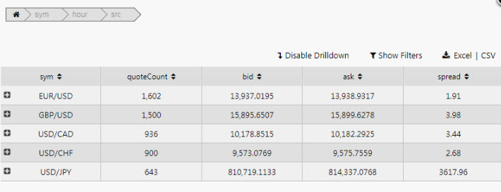
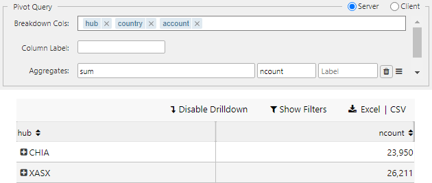
The following screenshot shows a standard pivot using the above query.
- Standard Pivot
In the next screenshot you can see that Column Label has been set to displayQueue to create a 2D Pivot.
Navigation of a OLAP / Pivot control requires enabling Breadcrumbs in a component, or linking with a Breadcrumbs component.
Aggregate functions#
For Pivot Queries, you have the option to specify unary, binary or custom binary, aggregate analytics.
The following sections provide examples where select from dfxQuote is the query and Pivot is checked.
- Unary analytics- takes a single input (Un)
- Binary analytics- takes two inputs (Bi)
- Custom binary analytics- take two inputs and performs a specific custom user-defined computation on them
In the Pivot Query panel the following fields are set:
- Breakdown Cols - The drill-down buckets, i.e. the independent variables
- Aggregates - These are functions of the dependent variables. Unary functions are
sum,avg,count,min,max.
Unary analytic#
The following screenshot shows an example of a unary analytic.
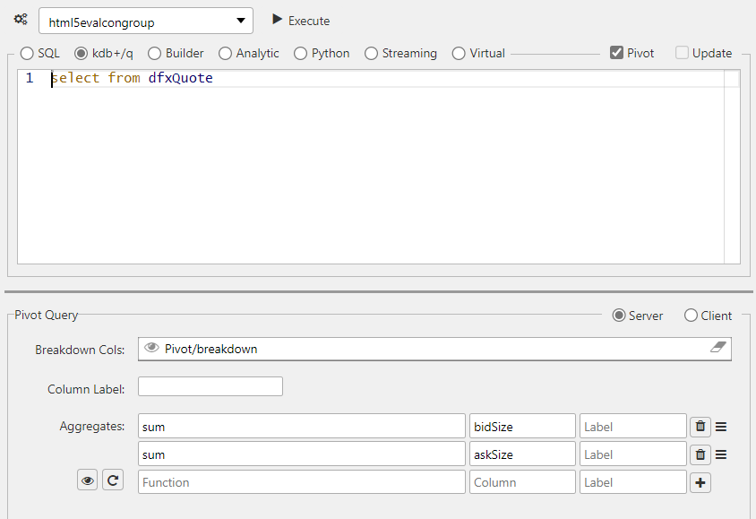
In this example the single input sum is used.
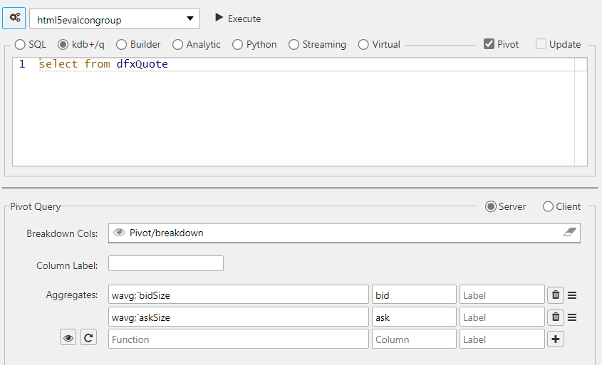
Binary analytic#
The following screenshot shows an example of a binary analytic.
Custom binary analytics#
In addition to the built-in functions, such as sum, avg, count, min, max, you can define custom binary functions that take two inputs and performs a specific custom user-defined computation on them.
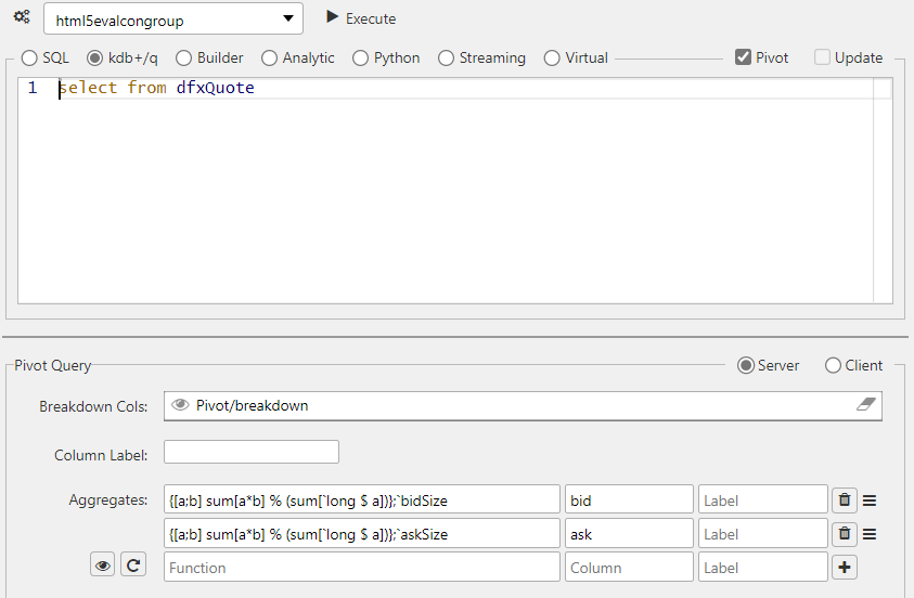
Example
A standard built-in binary function is available as part of the VWAP Analytic (subVWAP) found in Demo Trading dashboard in the Dashboard evaluation pack. bSize is bid size. In this example the dividend is defined as the sum of the bidSize value multiplied bid value and the divisor is defined by converting the bidSize to long and get the sum of these long values.
q
{[a;b] sum[a*b] % (sum[`long $ a])};`bidSize
Dynamic aggregate columns#
Dynamic aggregate columns for pivot queries typically refers to a situation where you want to aggregate data dynamically based on certain conditions or parameters using view states (rather than hard-coding the aggregates). This is particularly useful when you have varying requirements for aggregation depending on the data or when you want the query to be adaptable to changes in the dataset
To enable, click the View State icon in the basic pivot query control.
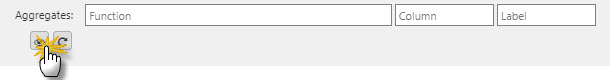
You can use view states to define Breakdown columns, Aggregate Columns, Aggregate Functions and Labels. Each view state must be of type list and each Aggregate Column must have a corresponding Aggregate function.
Remember to link to a Breadcrumbs component for navigation control of the pivot.
Update query#
An update query allows a user to make permanent changes to source data from the Data Grid. For example, when adding a new client or customer. The update query requires both a query, and a settings check in Data Grid properties.
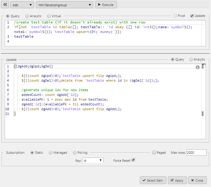
Keyed Tables
If using a keyed table then the query must use the same value.
Force Reset
To ensure updates are returned to the user view, Force Reset must be enabled.
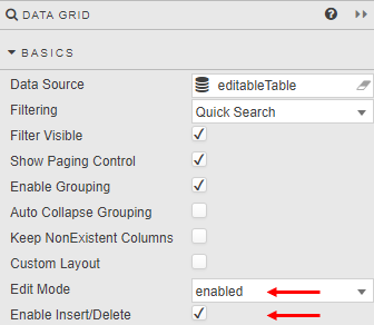
In addition to using an update query the Data Grid requires the following Basic properties to be set:
- Edit Mode to be enabled or instant
- Enable Insert/Delete to be checked.
The dashboard users then has an Edit option in their dashboard.
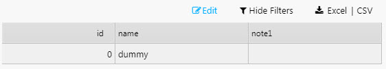
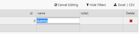
The dashboard user can make a change, as shown below.
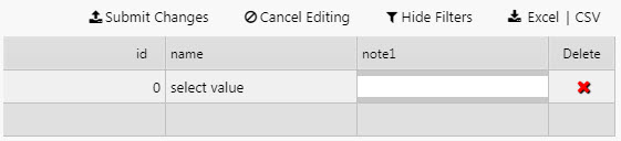
The dashboard user can submit a change, as shown below.
Permission to edit
If Update Query is enabled, all users with permissions for that dashboard can make changes. If you want only some read-only users to have edit permissions do the following:
- Duplicate the dashboard
- Set Edit Mode to disabled and uncheck Enable Insert/Delete from the Data Grid properties
- Grant users who shouldn’t have edit control permissions to access this duplicate dashboard.
Results#
When you click Execute on a data source query the results are displayed in the Results panel at the bottom of the screen. This panel has 3 tabs:
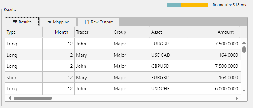
Performance metrics are also displayed to indicate query performance. The Roundtrip time, for the query to execute, is displayed in milliseconds above the results.
Results#
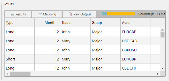
Results are displayed in the Results tab in the Results panel, as shown below.
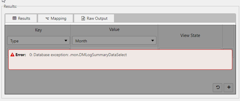
If the query does not execute an error is displayed, as shown below.
Mapping#
Mapping configuration is accessible from the Mapping tab in the Results panel, as shown below. Through this tab you can map results from a data source to view states.
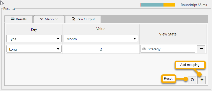
To create mappings, the results must include a column that contains keys and a column that contains values. Key and value columns are returned in the Key and Value dropdowns.
- Click + to add a new mapping.
-
Select a Key and specify the View State that the Value maps to.
- You can select Key values using the dropdowns or type them into the dropdown input field and press enter.
- Click the Reset icon to repopulate the list of mappings with all available keys.
Raw Output#
Raw output is displayed in the Raw Output tab in the Results panel. This information gives you further insights that maybe helpful for debugging. It presents exact unformatted data that is returned by the query.
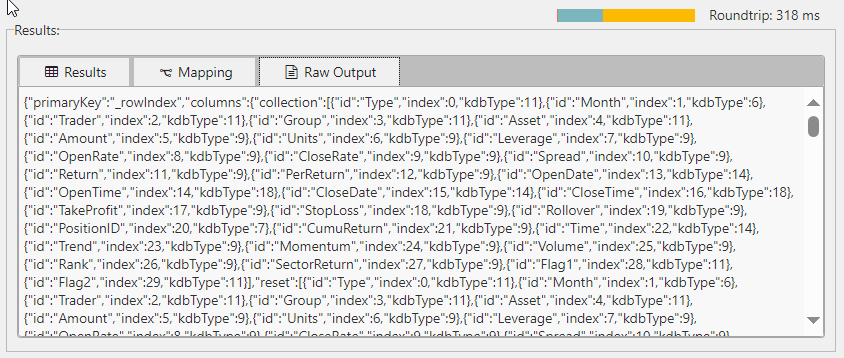
The raw data is comprised of the following elements:
- an array of column names
- an object mapping column names to their kdb types
- an array of row objects which map columns to values