3. Lists¶
3.0 Overview¶
All data structures in q are ultimately built from lists: a dictionary is a pair of lists; a table is a special dictionary; a keyed table is a pair of tables. Thus it is important to have a thorough grounding in lists.
All lists are equal but some lists are more equal than others. These are the lists of atoms of homogenous type, called simple lists – known in mathematics as vectors. They have optimum storage and performance characteristics.
While q’s list operations are similar to those in other functional languages, lists are stored and processed quite differently.
- They are not stored as singly-linked lists under the covers. Simple lists occupy contiguous storage and general lists are pointers in contiguous storage.
- Appending items to the end rather than “cons”-ing to the front.
- Efficient direct item access is available via indexing.
- A general list can hold items of different type without resorting to a union (sum) type.
It may be instructive to think of q lists as dynamically allocated arrays.
3.1 Introduction to Lists¶
A list is an ordered collection. “A collection of what?” you ask. More precisely, a list is recursively defined as an ordered collection of atoms and other lists. We pay special attention to the case in which the list comprises atoms of uniform type.
3.1.1 List Definition and Assignment¶
A (general) list is an ordered collection of q data. The members of the collection are its items. The notation for a general list encloses its items within matching parentheses and separates them with semi-colons.
Whitespace in list notation is optional. In what follows, we shall often insert optional whitespace after the semicolon separators for readability.
q)(1; 1.1; `1)
_
q)(1;2;3)
_
q)("a";"b";"c";"d")
_
q)(`Life;`the;`Universe;`and;`Everything)
_
q)(-10.0; 3.1415e; 1b; `abc; "z")
_
q)((1; 2; 3); (4; 5))
_
q)((1; 2; 3); (`1; "2"; 3); 4.4)
_
If you diligently entered each of these examples in your console, you have noticed that q does not always echo what you type. The initial and last three lists are general lists, meaning they are not homogenous atoms. This could mean atoms of mixed type, nested lists of uniform type, or atoms and nested lists of mixed type.
Items in a list are sequenced from left to right, providing an inherent order. The lists 1;2 and 2;1 are different. SQL is based on sets, which are inherently unordered. This distinction leads to some subtle differences between the semantics of queries on q tables versus the analogous SQL queries. The inherent ordering of lists makes large time series processing natural and fast in q, while it is cumbersome and slow in standard SQL due to the need to place things in order.
Lists can be assigned to variables exactly like atoms.
q)L1:(1;2;3)
q)L2:("z";"a";"p";"h";"o";"d")
q)L3:((1; 2; 3); (`1; "2"; 3); 4.4)
3.1.2 count¶
The number of items in a list is its count. You obtain the count of a list by asking for it with the unary function count.
q)count (1; 2; 3)
3
q)count L1
_
This is our first encounter with a q function (or keyword), which we will learn about in Chapters 4 and 5. For now, we need only understand that count returns a long equal to the number of items in the list to its right.
The maximum number of items for a list in q3.* is 264-1. In q2.* it was 2 billion.
Observe that the count of an atom is 1 even though an atom is not a list.
q)count 42
1
q)count `zaphod
_
Other useful operations are provided by first and last that return the first and last item in a list, respectively.
q)first (1; 2; 3)
1
q)last (1; 2; 3)
3
3.2 Simple Lists¶
A list of atoms of a uniform type, called a simple list, corresponds to the mathematical notion of a vector. Such lists are treated specially in q. They have a simplified notation, take less storage and compute faster than general lists.
You can always use general list notation, even for simple lists.
Whenever q recognizes that the items of a list are homogenous atoms, it dynamically converts to a simple list without asking for permission. In most cases, the storage and performance advantages justify the imposition. However, in some cases – such as deletion of an outlier item of non-uniform type – this can cause a programming headache because the list will no longer allow appends or updates with items that do not conform to the resulting uniform type.
3.2.1 Simple Integer Lists¶
The console display of a simple list of any numeric type omits the enclosing parentheses and replaces the separating semi-colons with (required) blanks. The following two expressions define the same list, as q verifies by testing for identity using ~.
q)(100;200;300)
_
q)100 200 300
_
q)100 200 300~(100; 200 ; 300)
1b
The console display of the first expression demonstrates the automatic conversion to simple lists previously mentioned.
Similar notation, with the addition of a single trailing type indicator, is used for simple lists of short and int.
q)(1h; 2h; 3h)
1 2 3h
q)(100i; 200i; 300i)
_
Trailing type indicator
The trailing type indicator in the console display of a simple list applies to the entire list and not just the last item of the list; otherwise, the list would not be simple and would be displayed in general form:
q)(1; 2; 3h)
1
2
3h
3.2.2 Simple Floating Point Lists¶
Simple lists of float and real are notated the same as integral lists.
q)(123.4567; 9876.543; 99.0)
123.4567 9876.543 99
q)123.4567 9876.543 99
_
Observe that the q console suppresses the decimal point when displaying a float having zero(es) to the right of the decimal; but the value is not an integer. This notational efficiency for float display means that a list of floats having no decimal parts displays with a trailing ‘f’.
q)1.0 2.0 3.0
1 2 3f
q)1 2 3f~1.0 2.0 3.0
_
Also observe that if you include what appears to be an integer in a list of float, q assumes that you are following its convention by merely omitting redundant data to the right of the decimal. That is, you get a list of float and not a general list.
q)1.1 2 3.3~1.1 2.0 3.3
_
3.2.3 Simple Binary Lists¶
The abbreviated notation for a simple list of boolean or byte data juxtaposes the individual data values together with no whitespace between. The b type indicator for boolean trails the list.
q)(0b;1b;0b;1b;1b)
01011b
q)01011b
_
Storage for a simple boolean list
A simple list of boolean atoms requires the same number of bytes to store as it has atoms. While the simplified notation is suggestive of a bit mask, multiple bits are not compressed to fit inside a single byte. The boolean list above uses 5 bytes of storage.
The 0x indicator for a simple list of byte precedes the list.
q)(0x20;0xa1;0xff)
0x20a1ff
q)0x20a1ff~(0x20;0xa1;0xff)
_
The display of a simple list of GUIDs is the same is that of integers – i.e., the values are separated by spaces.
q)3?0Ng
_
3.2.4 Simple Symbol Lists¶
The abbreviated notation for simple lists of symbols juxtaposes the individual atoms with no intervening whitespace.
q)(`Life;`the;`Universe;`and;`Everything)
`Life`the`Universe`and`Everything
q)`Life`the`Universe`and`Everything
_
Inserting spaces between symbol atoms causes an error.
q)`bad `news
'bad
3.2.5 Simple char Lists and Strings¶
The simplified notation for a list of char looks just like a string in most languages, with the juxtaposed sequence of characters enclosed in double quotes.
q)("s"; "t"; "r"; "i"; "n"; "g")
"string"
q)"string"
_
A simple list of char is actually called a string; however, it does not have the atomic semantics of a string in most languages. Since it is a list of char, not an atom, you cannot ask if two strings of different lengths are equal. You can ask if they are identical (as you can with any two q entities).
q)"string"="text"
'length
q)"string"~"text"
0b
3.2.6 Lists of Temporal Data¶
Since they are really integers, the abbreviated form for simple temporal lists separates items with a space.
q)(2000.01.01; 2001.01.01; 2002.01.01)
_
q)(00:00:00.000; 00:00:01.000; 00:00:02.000)
_
Specifying a list of mixed temporal types has a different behavior from that of a list of mixed numeric types. In this case, the list takes the type of the first item in the list; other items are widened or narrowed to match.
Mixed lists cannot be written in the vector notation
The paragraph above is in error.
By definition, vectors have uniform type. The temporal vector notation allows items to be written in the notation of a narrower type, which the parser silently widens. The next example demonstrates this. — Editor
q)12:34 01:02:03
12:34:00 01:02:03
q)01:02:03 12:34
_
To force the type of a mixed list of temporal values, append a type specifier.
q)01:02:03 12:34 11:59:59.999u
01:02 12:34 11:59
3.3 Empty and Singleton Lists¶
Lists with one or zero items merit special consideration, especially since q’s notation and display are not exactly intuitive.
3.3.1 The General Empty List¶
It is useful to have lists with no items. A pair of parentheses enclosing nothing (except optional whitespace) denotes the general empty list, which (annoyingly) has no console display.
q)()
q)
We shall see in §7.4 that it is possible to define an empty list with a specific type, so that only items of that type can be added to it.
Advanced
If you want to force the display of an empty list, use the q utility .Q.s1, which converts any q entity into a string suitable for display. Perhaps this utility should be called the “wizard of Oz” operator since it reveals what’s behind the curtain.
q)L:()
q)L
q).Q.s1 L
"()"
3.3.2 Singleton Lists¶
A singleton is a list containing a single item. As any postal clerk will tell you, an item in a box is not the same as an unboxed item. So an atom and a singleton containing that atom are different.
The syntax of a singleton presents a notational conundrum for q. We might expect to write the singleton list containing 42 as (42) but we cannot. The issue arises from q’s use of parentheses both for list demarcation and for the usual mathematical grouping in expressions. The latter leads to the following sequence of arithmetic reductions.
(40+2) (42) 42
This forces (42) to be the atom 42.
Unfortunately, there is no way to type a singleton literal. Singletons are created by the function enlist, which “boxes” its argument into a list with one item. Note that it manages to avoid the usual q predilection for aggressively short names.
q)enlist 42
,42
Observe that the console display of a singleton list uses the k form of enlist – i.e., unary ,. Don’t be fooled: we can’t use this in q.
Single-character strings
A string with a single character cannot be written syntactically as “a” – this is a character atom. Use enlist. This is a common error for qbies.
q)"a"
_
q)enlist "a"
_
A singleton need not contain an atom as its sole item; it can be any q entity.
q)enlist 1 2 3
1 2 3
q)enlist (10 20 30; `a`b`c)
10 20 30 a b c
Observe that the console display is not consistent with showing , and sometimes is downright confusing.
3.4 Indexing¶
A list is sequenced from left-to-right in the position of its items. The offset of an item from the beginning of the list is called its index. The initial item has index 0, the second item has index 1, etc. Thus a list of count n has items at indices 0 through n - 1.
There is no item at index n. This is a common qbie mistake.
3.4.1 Index Notation¶
To access the item at index i in a list, follow the list immediately with [i]. This is called item indexing. For example,
q)(100; 200; 300)[0]
100
q)100 200 300[0]
100
q)L:100 200 300
q)L[0]
100
q)L[1]
_
q)L[3] / index out of bounds returns null value
_
q)L[2]
_
3.4.2 Indexed Assignment¶
Items in a list can also be assigned via item indexing. Thus,
q)L:1 2 3
q)L[1]:42
q)L
1 42 3
Index assignment into a simple list
Index assignment into a simple list enforces strict type matching with no type promotion. Otherwise put, when you assign an item into a simple list, the type must match exactly – i.e., a narrower type is not widened.
q)L:100 200 300
q)L[1]:42h
'type
This may come as a surprise if you are accustomed to numeric values always being promoted in a dynamically typed language – e.g., q itself.
Should you find exceptions to this in some releases of q3.*, do not count on them being there in future releases!
3.4.3 Indexing Domain¶
Providing an invalid data type for the index results in an error.
q)L:(-10.0; 3.1415e; 1b; `abc; "z")
q)L[1.0]
'type
In contrast, if you index outside the proper bounds of the list, the result is not an error. Instead you get a null value, indicating “missing data.” Specifically, indexing outside the range of 0 to (count L) – 1 yields a null of the type of the item at index 0. This is the most efficient thing to return in the case of a general list where there is no canonical item type.
q)L1:1 2 3 4
q)L1[4]
0N
q)L2:1.1 2.2 3.3
q)L2[-1]
0n
q)L3:(`1; 2; 3.3)
q)L3[0W]
`
Pay special attention to the first example above that indexes the list at its count. Indexing one position past the end of the list is easy for qbies, especially if you’re not accustomed to indexing relative to 0.
3.4.4 Empty Index and Null Item¶
An omitted index returns the entire list.
q)L:10 20 30 40
q)L[]
10 20 30 40
An omitted index is not the same as indexing with an empty list. The latter returns an empty list, so we use the .Q.s1 utility to reveal its display.
q).Q.s1 L[()]
"()"
The syntactic form double-colon :: denotes the nil item, which allows explicit notation or programmatic generation of an empty index.
q)L[::]
_
Including the nil item in a list
The type of the nil item does not match any other type in q. Consequently, inclusion of the nil item in a list forces the list to be general.
q)L:(::; 1 ; 2 ; 3)
q)type L
0h
q).Q.s1 L[0]
"::"
This is one way to avoid a nasty surprise when q would otherwise automatically convert a list to simple type. A simple case is when you reassign the only non-conforming item in the list.
q)L:(1; 2; 3; `a)
q)L[3]:4
q)L
1 2 3 4
q)L[3]:`a
'type
After the reassignment you can no longer assign `a back into the list in its original position. One way to avoid this is by placing :: in the list as a guard.
q)L:(::; 1 ; 2 ; 3; `a)
q)L[4]:4
q)L[4]:`a
q)
A drawback of this technique is that you must avoid passing :: on to expressions that use the actual data in the list.
3.4.5 Lists with Expressions¶
Any valid q expression can occur in list construction.
q)a:42
q)b:43
q)(a; b)
42 43
q)L1:1 2 3
q)L2:40 50
q)(L1; L2)
q)(count L1; sum L2)
_
You cannot use the abbreviated notation of simple lists with variables.
q)a:42
q)b:43
q)a b
': Bad file descriptor|
The reason for this cryptic error message will be apparent when we deal with files later.
3.5 Combining Lists¶
3.5.1 Joining with ,¶
We scoop the presentation on operators in the next chapter to describe the Join operator ,. Its result is a new list in which (a copy of) the right operand is appended to the end of (a copy of) the left operand. Join accepts an atom in either argument – i.e., as if the corresponding singleton had been supplied.
q)1 2 3,4 5
1 2 3 4 5
q)1,2 3 4
1 2 3 4
q)1 2 3,4
1 2 3 4
Observe that if the arguments are not of uniform type, the result is a general list.
q)1 2 3,4.4 5.5
_
Ensuring a list
To ensure that a q entity becomes a list, use either (),x or x,(). This leaves a list unchanged but effectively enlists an atom. Such a seemingly trivial expression is actually useful and is our first example of a q idiom. You cannot use enlist x for the same purpose. Why not?
3.5.2 Merging with ^¶
Another way to combine two lists of the same length is by coalescing them with ^. The result is given by the rule that the right item prevails over the corresponding left item except when the right item is null.
q)L1:10 0N 30
q)L2:100 200 0N
q)L1^L2
100 200 30
3.6 Lists as Maps¶
Thus far, we have considered a list as data – i.e., a static collection of its items. We can also view it as a mathematical mapping provided by item indexing. Specifically, a list provides a map whose domain is integers and whose codomain is the collection of its items (supplemented with a null value). The list map assigns the output value L[i] to the input value i.
i | – > L[i]
Here are the I/O tables for some basic lists.
101 102 103 104| I | O |
|---|---|
| 0 | 101 |
| 1 | 102 |
| 2 | 103 |
| 3 | 104 |
(`a; 123.45; 1b)| I | O |
|---|---|
| 0 | `a |
| 1 | 123.45 |
| 2 | 1b |
(1 2; 3 4)| I | O |
|---|---|
| 0 | 1 2 |
| 1 | 3 4 |
The codomains of the first two examples are collection of atoms. The last example has a codomain comprised of lists.
A list not only acts like a map, it is a unary map whose notation is the same as function application. This is a useful way of looking at things. We shall see in Chapter 4 that a nested list can be viewed as a multivalent map.
From the perspective of lists as maps, the fact that indexing outside the bounds of a list returns a null means the map is implicitly extended to the domain of all integers with null output value outside the list proper.
3.7 Nesting¶
Data complexity is built by using lists as items of lists.
3.7.1 Depth¶
Now that we’re comfortable with simple lists, we return to general lists. Nested lists have item(s) that are themselves lists. The number of levels of nesting for a list is called its depth. Informally, the depth measures how much repeated indexing is necessary to arrive at only atoms. Atoms have depth 0 and simple lists have depth 1.
The notation of complex lists is reflected in nested parentheses. For pedagogical purposes, in this section only, we shall often use general notation to define even simple lists since the parentheses make things manifest. However, the console always displays lists in the most concise form.
Following is a list of depth 2 that has three items, the first two being atoms and the last a list. We also show its simplified notation.
q)L:(1;2;(100;200))
q)count L
_
q)L:(1;2;100 200)
_
q)count L
3
q)L[0]
_
q)L[1]
_
q)L[2]
100 200
3.7.2 Pictorial Representation¶
We present a pictorial representation that may help in visualizing levels of nesting. An atom is represented as a circle containing its value. A list is represented as a box containing its items. A general list is a box containing boxes and atoms.
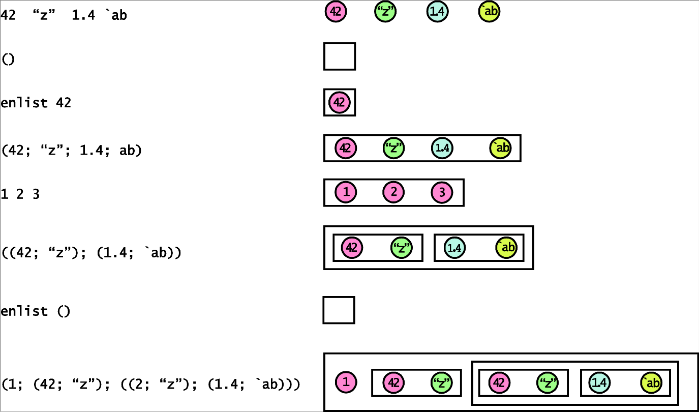
3.7.3 Examples¶
Following is a list of depth 2 with two elements, each of which is a simple list.
q)L2:((1;2;3);(`ab;`c))
q)count L2
_
Following is a list of depth 2 having three elements, two of which are general lists and one is an atom.
q)L3:((1; 2h; 3j); ("a"; `bc`de); 1.23)
q)count L3
_
q)L3[1]
_
q)count L3[1]
_
Following is a list of depth 2 having one item that is a simple list.
q)L4:enlist 1 2 3 4
q)count L4
_
q)count L4[0]
_
Following is a “rectangular” list that can be thought of as the 3×4 matrix its display resembles.
q)m:((11; 12; 13; 14); (21; 22; 23; 24); (31; 32; 33; 34))
q)m
11 12 13 14
21 22 23 24
31 32 33 34
q)m[0]
_
q)m[1]
_
q)m[1][0]
3.8 Iterated Indexing and Indexing at Depth¶
In the examples above, we saw that the display of nested lists suggests arrays from other languages. You can indeed think of them as “ragged” arrays, as long you are careful about the iterated indexing. Indexing at depth is an alternate notation that suggests nested lists can also be viewed as higher-dimensional arrays.
3.8.1 Iterated Item Indexing¶
Retrieving an item in a nested list via a single index retrieves a top-most item.
q)L:(1; (100; 200; (1000; 2000; 3000; 4000)))
q)L[0]
_
q)L[1]
100
200
1000 2000 3000 4000
Interpreting list indexing as function application for positional retrieval, we can read the last line,
Retrieve the item at index 1 from L
Since the result L[1] is itself a list, we can also retrieve its items via indexing. For example,
q)L[1][2]
1000 2000 3000 4000
Read this as,
Retrieve the item at index 2 from the item at index 1 in L
We can once again index into this result.
q)L[1][2][0]
1000
Read this as,
Retrieve the item at index 0 from the item at index 2 in the item at index 1 in L
3.8.2 Indexing at Depth¶
There is an alternate notation for iterated indexing into a nested list. It is strictly syntactic sugar and amounts to the same thing under the covers. This notation is called indexing at depth and it looks exactly like application of a multi-valent function (which, in fact, it is). The previous retrieval can also be written as,
q)L[1;2;0]
_
From one point of view, indexing at depth simplifies the notation for retrieval of inner items from a nested list.
Semicolons in indexing
The semicolons in indexing at depth notation might make it appear that the collection of indices is a list. It is not, although we shall see later a way to perform indexing at depth in which the indices are a list. Also, don’t confuse the semicolons with commas, which is a common qbie mistake.
Assignment via index at depth works but assignment does not work with iterated indexing.
q)L:(1; (100; 200; (1000 2000 3000 4000)))
q)L[1; 2; 0]: 999
q)L
_
q)L[1][2][0]:42
'assign
The last expression fails essentially because the intermediate retrievals are ephemeral – i.e., they not addressable entities.
To confirm that the notation for indexing at depth is reasonable, we return to our “matrix” example.
q)m:((11; 12; 13; 14); (21; 22; 23; 24); (31; 32; 33; 34))
q)m
_
q)m[0][0]
11
q)m[0; 0]
11
q)m[0; 1]
_
q)m[1; 2]
_
The indexing at depth notation suggests thinking of m as a multi-dimensional matrix, whereas repeated single indexing suggests thinking of it as an array of arrays. Chacun à son goût.
Take specifying only number of rows (or columns)
It is possible to create a (possibly ragged) array of a given number of rows or columns from a flat list using the reshape operator # by specifying 0N (missing data) for the number of rows or columns in the left operand.
q)2 0N#til 10
0 1 2 3 4
5 6 7 8 9
q)0N 3#til 10
0 1 2
3 4 5
6 7 8
,9
3.9 Indexing with Lists¶
As a vector language, q prefers to deal with lists whenever possible. To this end, there is no reason to restrict list retrieval to one item at a time. Instead, we can ask for a list of items by passing a list of indices.
3.9.1 Retrieving Multiple Items¶
In this section, we begin to see the power of q as a vector language. We start with,
q)L:100 200 300 400We know how to index single items of the list.
q)L[0]
100
q)L[2]
_
By extension, we can retrieve a list of multiple items via multiple indices. For simplicity we use simple list notation for the indices.
q)L[0 2]
100 300
The indices can be in any order, or even be duplicated and the corresponding items are retrieved. The shape of the output conforms to the input.
q)L[3 2 0 1]
_
q)L[0 2 0]
_
Here are some examples of indexing into literal lists.
q)01101011b[0 2 4]
011b
q)"beeblebrox"[0 7 8]
_
Getting the semi-colons right
Using a list as an index demonstrates why getting the semi-colon separators right is essential when indexing at depth. Leaving them out or using commas effectively specifies multiple indices, and you will get a corresponding list of values from the top level.
3.9.2 Indexing via a Variable¶
When retrieving items via multiple indices, the indices can live in a variable.
q)L
100 200 300 400
q)I:0 2
q)L[I]
100 300
3.9.3 Indexing with Nested Lists¶
Observe that in our examples of list indexing, the result of index retrieval has the same shape as the index. If the index is an atom the result is an atom. When the index list was a simple list, the result was a list of the same count.
More generally, we can retrieve via an arbitrary collection of indices. The retrieved list has the same shape as the index list.
q)L:100 200 300 400
q)L[(0 1; 2 3)]
100 200
300 400
Do not confuse this with indexing at depth. In the present case all items are retrieved at the top level only
Advanced: result conforms to index
More precisely, the result of indexing via a list conforms to the index list.
The notion of conformability of lists is defined recursively. All atoms conform. Two lists conform if they have the same number of items and each of their corresponding items conform. In plain language, two lists conform if they have the same shape.
3.9.4 Assignment with List Indexing¶
Recall that a list item can be (re)assigned via item indexing,
q)L:100 200 300 400
q)L[0]:100
q)L
_
Assignment via index extends to indexing via a simple list with the proviso that the index list and value list conform.
q)L[1 2 3]:2000 3000 4000
q)L
_
Assignment via a simple index list is processed in sequence – i.e., from left-to-right. Thus,
q)L[3 2 1]:999 888 777
is equivalent to,
q)L[3]:999
q)L[2]:888
q)L[1]:777
Consequently, in the case of a repeated item in the index list (not a swell idea), the right-most assignment prevails.
q)L:100 200 300 400
q)L[0 1 0 3]:1000 2000 3000 4000
q)L
_
You can assign a single value to multiple items in a list by using an atom for the assignment value. This is an example of a general phenomenon in q in which an atom is extended to conform to a list.
q)L:100 200 300 400
q)L[1 3]:999
q)L
_
3.9.5 Juxtaposition¶
Now that we’re familiar with retrieving and assigning via an index list, we introduce a simplified notation that is common in functional programming. It is permissible to leave out the brackets and juxtapose the list and index with separating whitespace (usually just a blank). Some examples follow.
q)L:100 200 300 400
q)L[0]
100
q)L 0
100
q)L[2 1]
_
q)L 2 1
_
q)I:2 1
q)L I
_
q)L ::
_
In the colloquial, “We don’t need no stinkin’ brackets!”
Which notation you use is a matter of personal preference. In this tutorial, we initially use brackets, since this notation is probably most comfortable for qbies coming from traditional programming. Experienced q programmers often use prefix syntax since it reduces notational density, although brackets can eliminate some parentheses.
3.9.6 Find (?)¶
The Find operator is (an overload of) binary ? that returns the index of the first occurrence of the right operand in the left operand.
q)1001 1002 1003?1002
1
Since Find maps an item to its index, it is inverse to indexing – i.e., list positional retrieval thought of as a mapping.
If you try to find an item that is not in the list, the result is an integer equal to the count of the list.
q)1001 1002 1003?1004
3
One way to think of this result is that the position of an item that is not in the list is one past the end of the list, which is where it would be if you were to append it to the list.
Find is atomic in the right operand meaning that it extends to lists.
q)1001 1002 1003?1003 1001
_
3.10 Elided Indices¶
3.10.1 Eliding Indices for a Matrix¶
We return to the situation of indexing at depth for nested lists. For simplicity, we start with a rectangular list that displays as a matrix.
q)m:(1 2 3 4; 100 200 300 400; 1000 2000 3000 4000)
q)m
_
Analogy with traditional matrix notation suggests that we could retrieve a row or column from m by providing a “partial” index at depth. This indeed works because eliding an index in any slot is equivalent to specifying all legitimate indices for that slot.
q)m[1;]
100 200 300 400
m[;3]
4 400 4000
Observe that eliding the last index reduces to item indexing at the top level.
q)m[1;]~m[1]
_
Because of this correspondence, it is permissible to drop the trailing semicolon. We recommend against this practice as it makes the purpose of code less evident.
The situation of eliding the first index is more interesting. It essentially retrieves a “column” as a slice through the top-level lists – i.e., a row.
3.10.2 Eliding Indices for Deeply Nested Lists¶
Let’s tackle three levels of nesting. Here we can elide one or two indices in any slots.
q)L:((1 2 3;4 5 6 7);(`a`b`c`d;`z`y`x`;`0`1`2);("now";"is";"the"))
q)L
(1 2 3;4 5 6 7)
(`a`b`c`d;`z`y`x`;`0`1`2)
("now";"is";"the")
q)L[;1;]
4 5 6 7
`z`y`x`
"is"
q)L[;;2]
3 6
`c`x`2
"w e"
Interpret L[;1;] as,
Retrieve all items at index 1 of each top level list
Interpret L[;;2] as,
Retrieve the items at index 2 for each list at the second level
Observe that in L[;;2] the attempt to retrieve the item at index 2 of the string "is" was out of bounds and so resulted in the null value " ". This is the source of the blank in "w e" of the result.
As the final exam for this section, let’s combine an elided index with indexing by lists to retrieve a cross-section of L. Try to predict the result before entering the expression into your console session.
q)L[0 2;;0 1]
_
Interpret this as,
Retrieve the items at positions 0 and 1 from all columns in rows 0 and 2
Style Recommendation
In general, it is permissible to elide all trailing semicolons arising from elided indices. We consider this bad practice. Looking at the notation below, would you guess that the expression after the comment arose from that to the left of it? We didn’t think so.
L[1;;] / instead of L[1]
L[;1;] / instead of L[;1]
3.11 Rectangular Lists and Matrices¶
3.11.1 Rectangular Lists¶
In this section, we further investigate matrix-like nested lists. A rectangular list is a list of lists all having the same count. This does not mean that a rectangular list is necessarily a traditional matrix, since there can be additional levels of nesting.
q)L:(1 2 3; (10 20; 100 200; 1000 2000))
q)L
1 2 3
10 20 100 200 1000 2000
A rectangular list can be transposed with flip, meaning that the rows and columns are reflected across the diagonal. When flip is applied to a rectangular list, it physically transposes the data – i.e., it allocates new storage and copies the original data in column order.
q)L:(1 2 3; 10 20 30; 100 200 300)
q)L
1 2 3
10 20 30
100 200 300
q)flip L
1 10 100
2 20 200
3 30 300
This effectively reverses the first and second slots in indexing at depth.
q)L:(1 2 3; 10 20 30; 100 200 300)
q)M:flip L
q)L[1;2]
30
q)M[2;1]
30
3.11.2 Formal Definition of Matrices¶
Matrices are a special case of rectangular lists and are defined recursively. A matrix of dimension 0 is a scalar. A matrix of dimension 1 is a simple list – i.e., a vector. The count of a vector is usually called its length or dimension in mathematics. Some functional programming languages have tuples, which can be thought of as coordinates of fixed-dimension vectors with respect to a basis; q does not.
In q, vectors do not need to be of numeric type.
q)v1:1 2 3 / vector of integers
q)v2:98.60 99.72 100.34 101.93 / float vector
q)v3:`so`long`and`thanks`for`all`the`fish / symbol vector
For n>1, we define a matrix of dimension n as a list of matrices of dimension n - 1 all having the same size. Thus, a matrix of dimension 2 is a list of vectors, all having the same size. If all atoms in a matrix have the same type, we call this the type of the matrix.
3.11.3 Two- and Three-Dimensional Matrices¶
Let m be a two-dimensional matrix as defined in the previous section. The items of m are its rows. As we have already seen, the ith row of m can be obtained via item indexing as m[i]. Equivalently, we can use an elided index with indexing at depth to obtain the ith row as m[i;].
The console display of m in tabular form motivates defining the list m[;j] as the jth column of m. The notations m[i][j] and m[i;j] both retrieve the same item – namely, the item in row i and column j.
We make one final observation. Matrices are nested lists stored in row order. When the rows are simple, each occupies contiguous storage. This makes row retrieval very fast. On the other hand, columns must be picked out of the rows, so column operations are slower.
Advanced
By convention we consider a matrix to be a collection of rows. It would be equally valid to consider each vector as a column and a two dimensional array as a collection of columns. As we shall see in Chapter 8, a table is a collection of columns that are logically (not physically) transposed for ease of indexing. The constraints and calculations of q-sql operate on table column lists, so they are fast, especially when the columns are simple lists. In particular, a simple time series can be represented by two parallel lists, one holding temporal values and the other holding the associated values. Retrieving and manipulating the columns in vector operations is faster by orders of magnitude than performing the same operations in an RDBMS that stores data in rows with undefined order.
Higher-dimensional matrices occur less frequently in q than in its ancestors. For completeness, here is an example of a three-dimensional 2×3×2 matrix – i.e., each of the two top-level items is a 3×2 matrix. Observe that the console display of mm is unenlightening.
q)mm:((1 2;3 4;5 6);(10 20;30 40;50 60))
q)mm
_
q)mm[0]
_
q)mm[1]
_
3.11.4 Matrix Flexibility¶
We have seen that although there is no separate construct for matrices in q, rectangular lists look and act like their mathematical matrix counterparts. However, they have features not available in simple mathematical notation or in most traditional languages. We have seen that a rectangular list can be viewed and manipulated both as a multi-dimensional array (i.e., indexing at depth) and as an array of arrays (repeated item indexing). In addition, we can extend individual item indexing with indexing via lists.
q)m:(1 2; 10 20; 100 200; 1000 2000)
q)m 0 2
_
3.12 Useful List Operations¶
In this section we demonstrate basic use cases for some list operations that are frequently used in following chapters.
3.12.1 til¶
The unary til takes a non-negative integer n and returns a list of n consecutive natural numbers starting at 0. It is useful for constructing regular lists of integers.
q)til 10
0 1 2 3 4 5 6 7 8 9
q)1+til 10
_
q)2*til 10
_
q)1+2*til 10
_
q)-5+4*til 3
_
If your code includes constructs of the form function each til count …you are almost certainly writing loopy – i.e., non-vector – code, otherwise known as VBQ.
3.12.2 distinct¶
The unary function distinct returns the unique items in its list argument, in order of first occurrence.
q)distinct 1 2 3 2 3 4 6 4 3 5 6
1 2 3 4 6 5
3.12.3 where¶
The basic form of where returns the indices of 1b in a boolean list – i.e., it reports where the ones are.
q)where 101010b
0 2 4
This is useful to operate at positions that are indentified by a predicate.
q)L:10 20 30 40 50
q)L[where L>20]:42
q)L
_
3.12.4 group¶
The unary function group takes a list and returns a dictionary in which each distinct item of the argument is mapped to the indices of its occurrences, in order of occurrence.
q)group "i miss mississippi"
i| 0 3 8 11 14 17
 | 1 6
m| 2 7
s| 4 5 9 10 12 13
p| 15 16